Pooja S Dodamani^*and Ajit Danti

CSE, Christ University, Bangalore, 560057, India.

Corresponding Author E-mail: puja.pooh91@gmail.com

DOI : https://dx.doi.org/10.13005/bpj/2676

Abstract

The key focus of the current study is implementation of an automated semantic segmentation model to localize and extract bone regions from digital X-ray images. Methods: The proposed segmentation framework uses a pre-processing stage which follows convolutional neural network (CNN) obtained segmentation stage to extract the bone region from X-ray images, mainly for diagnosing critical conditions such as osteoporosis. Since the presence of noise is critical in image analysis, the X-ray images are initially processed with a grey wolf optimization (GWO) guided non-local means (NLM) denoising. The segmentation stage uses a Multi-Res U-Net architecture with attention modules. Findings: The proposed methodology shows superior results while segmenting bone regions from real X-ray images. The experiments include an ablation study that substantiates the need for the proposed denoising approach. Several standard segmentation benchmarks such as precision, recall, Dice-score, specificity, Intersection over Union (IOU), and total accuracy have been used for a comprehensive study. The proposed architectural has good impact compared to the state-of-the-art bone segmentation models and is compared both quantitatively and qualitatively. Novelty: The denoising using GWO-NLM adaptively chose the denoising parameters based on the required conditions and can be reused in other medical image analysis domains with minimal finetuning. The design of the proposed CNN model also aims at better performance on the target datasets.

Keywords

Convolutional neural network; Grey wolf optimization; Multi-Res U-Net; Non-local means denoising; Semantic segmentation

Download this article as: 

Copy the following to cite this article: Dodamani P. S, Danti A. Grey Wolf Optimization Guided Non-Local Means Denoising for Localizing and Extracting Bone Regions from X-Ray Images. Biomed Pharmacol J 2023;16(2).

Copy the following to cite this URL: Dodamani P. S, Danti A. Grey Wolf Optimization Guided Non-Local Means Denoising for Localizing and Extracting Bone Regions from X-Ray Images. Biomed Pharmacol J 2023;16(2). Available from: https://bit.ly/41gnIuD

Introduction

Recent advances in computer technology, machine learning, and the popularity of deep learning algorithms accelerated faster and more accurate image analysis, which eventually facilitated the popularity of computer-aided diagnosis (CAD). Identification, localization, and quantification of the region of interest is critical in medical diagnosis, and machine vision or image processing using machine learning is usually looking forward to boosting the perfection of automated decision-making.

Image segmentation refers to a broad research domain that helps to localize and extract the field of interest and is an important part of automated medical diagnosis. Identifying specific entities (like bone structures, lesions, blood vessels, etc.) from the images we are working with can be achieved only after gaining a good understanding of their unique features and experience over time. Recent years have seen significant advancements in the image quality, acquisition time and cost-effectiveness of well-known medical imaging methods such as computed tomography (CT) scan, X-ray imaging, magnetic resonance imaging (MRI) and ultrasonography (USG) [1]. However, these modalities have its own drawbacks mainly motion artifacts, noise, registration errors and contrast variations, leading to poor decision-making unless image processing algorithms specially equipped to address these issues. The most known applications include denoising, image registration, segmentation and classification.

Earlier, image segmentation approaches centered on unsupervised machine learning techniques mainly clustering and thresholding which may not require massive training data or ample computational resources [2]. Nevertheless, the increased complexity and demand for medical imaging data has evolved algorithms towards general feature extraction, that has raised the necessity for supervised machine learning techniques. Earlier, traditional most commonly used supervised machine learning models could learn generalized features from small, labeled datasets using handcrafted feature representations. However, it demands experts with superior domain knowledge, making human intervention inevitable. Since the learning depends highly on the reliability of the feature vectors, the models may not be reusable.

Research on decision-making using neural networks has been started from the second half of 20^th century. Numerous problems were faced earlier due to a lack of adequate data with high-performance computing. However, increased digital data accessibility and breakthroughs in GPU capabilities accelerated growth in the development of neural network algorithms. With the growing importance of imaging data in digital data pool, research has been further extended to convolutional neural networks (CNNs)[3]. The breakthroughs in CNN also benefited the medical image processing domain, mainly in the areas of segmentation and classification. Likewise, several convolutional neural networks based medical image segmentation techniques have been reported in the survey.

Diagnosis based on bone or similar hard tissue segmentation is comparatively lesser, and hence most of the research articles in the biomedical image segmentation domain focus on other predominant imaging modalities such as CT or MRI images rather than X-ray images. X-ray images are also susceptible to noise and contrast variations. Image quality in terms of pixel resolution is also critical in X-ray image analysis. Moreover, segmentation of the bone regions from similarly shaded soft tissues is also challenging. As a result, conventional machine learning models generally ineffective for segmenting X-ray images.

Unsupervised learning such as thresholding and clustering requires homogeneous pixel distribution, and the distinction between the foreground and background regions should be clear. Active contour-based models require manual intervention in marking the initial seed points, and such initialization may often require manual intervention from an expert. Improper feature extraction may create incorrect segmentation in the case of conventional supervised ML approaches.

Deep learning techniques can learn the image data adaptively and provide better accuracy, and the same is applicable in X-ray images as well. The key objective of current study is to develop and implement deep learning-based semantic segmentation model that can extract bone structures from digital X-ray images. This paper presents a novel CNN architecture that addresses several drawbacks of the traditional U-Net model [4], with proper integration of expert modules such as attention gates, residual blocks, and deep supervision. Additionally, the pipeline employs a customized denoising approach: GWO-NLM, allowing optimal denoising level adjustment during batch pre-processing of X-ray images.

The main section of this article is as follows: Section 2 elaborates analysis of relevant literature on existing bone segmentation techniques. Section 3 discusses about the proposed network architecture. Section 4 represents the experimental setup, results, and discussions. Last, Section 5 conclusion of this paper.

Literature Review

In this session, a survey on existing bone segmentation approaches has been conducted. Author proposed a mean-shift segmentation and an adaptive region merging algorithm to extract bone regions from X-ray images. Mean-shift clustering helps cluster the coarse level bone regions, and region merging helps identify the true boundaries. Though the approach is effective in good-quality X-ray images, the model is susceptible to image noise and contrast variations. An advanced version of the region growing method has been proposed[6] that uses multi-resolution wavelets and an active contour method. The study also uses a faster Hough transform to identify the diaphysis region from the extracted bone region[5].

Author segmented lateral skull images using a fuzzy set algorithm. Three distinct subsets are obtained by minimizing the known fuzzy index function: background, skin, and bones. As the similarity between two pixels increases, the fuzzy index function decreases. Due to the absence of spatial information, the segmented bone regions are disjoint and degrades the segmentation performance.[7]

Author presented a deep learning-based pediatric hand bone segmentation from X-ray images using a shallow layered U-Net based architecture. The model uses an encoder-decoder structure with depth-2 and variable kernel sizes for multi-scale image analysis. This work is one of the foremost hand bone region segmentation studies with deep learning these results show favorable performance in segmenting the bones from X-ray images acquired from children in different age groups.[8]

Author presented a machine learning approach to segment bone from X-rays, presented an end-to-end system that results in efficient and robust inference from small datasets. Their architecture: X-Net consists of multiple down sampling stage and up sampling stage in a single network. The multistage deconvolution stage entitles deviating the degrees of fine-grain feature level reconstruction mainly during upscaling, thus creating a denser feature space. The architecture is designed to perform more convolution on small datasets with minimal reduction in the boundary details. [8]

An approach which works on dilated residual based U-Net to segment the femur region and tibia bones region.[9] The model uses dilated convolution instead of standard known convolution to scale the depth of receptive field without max-pooling. A study estimating osteoporosis from X-ray images using a segmentation followed by a bone mineral density estimation. The model used a U-Net architecture with an attention gate mechanism to focus more on the bone regions. The above-discussed CNN models bear the native issue of U-Net, such as an unguaranteed focus on the region of interest and poor segmentation performance over the boundary areas. The proposed model investigates the drawbacks in the traditional encoder-decoder based CNN models, and addresses those issues by integrating appropriate modules to improve the bone segmentation.[11]

Methodology

The current study aims at segmenting bone regions from X-ray images that can be further processed to diagnose related critical illness conditions such as osteoporosis [12]. Since the quantification of the bone area is crucial in quantifying the bone mineral density (BMD), the segmentation quality should be fair enough to conduct further analysis. Hence the methodology is designed to improve the quality of the overall segmentation performance by integrating a novel denoising method for smoothing the image data followed by a deep learning-based segmentation. The overall pipeline is divided into two sub-processing stages. The initial stage will do a pre-processing stage to make the images in uniform pixel resolution and reduce noise from the raw input X-ray images. The latter stage uses the actual CNN-based semantic segmentation to extract bone regions from the soft tissue and background areas.

Pre-processing Stage

In this study, we have used X-ray images to segment the hard tissue bone regions [25]. The input images are acquired from various body parts such as chest, femur, ankle, etc., and hence generated with different pixel resolutions. The X-ray images may also be corrupted with noise and can make the segmentation task challenging. Hence the pre-processing part contains a resizing stage followed by a denoising stage for filtering the data for the subsequent segmentation stages.

Image Resizing

The X-ray images in the current study is of different resolution and a resizing operation is necessary to standardize the images for further analysis. Since the subsequent stage uses a CNN based segmentation, we resized all images to 512×512 resolution by considering various factors such as image quality, and computation complexity.

Image Denoising

X-ray images are often susceptible to various images noises such as speckle noise, impulse noise, and Poisson noise [13]. The type and amount of noise can vary widely depending on the hardware configuration; therefore, it is nearly impossible to expect low noise X-ray images. This demands an exclusive denoising stage prior to the main segmentation procedure. In this study proposes an improved non-local means (NLM) denoising [14], optimized using grey wolf optimization (GWO) [15] to filter the image with a proper trade-off among denoising level and computation time. The following sub-sections provide an in-depth discussion of the proposed grey wolf optimization-based non-local means (GWO-NLM) denoising stage.

An NLM filter’s denoising performance is generally determined by numerous hyperparameters such as search radius, kernel size and level of degrees of filtering. In general, these parameters are chosen empirically by weighing a variety of considerations such as the desired denoising region and computational cost. However, manually selecting these variables is challenging when processing a large image dataset. The choice of these several parameters has a serious impact on the weight of similarity between comparable blocks, which influences the denoising result. For example, a search space or large kernel increases the processing complexity, whereas a small sized kernel or search window may not remove noisy pixels within the needed range. As a result, automating the selection of these hyperparameters will aid in determining the ideal trade-off amongst the time complexity and denoising performance.

This paper presents an automatic parameter-based selection method for Non-Linear Means filters based on GWO. GWO assesses relevant combination of the Non-Linear Means parameters based on the obtained fitness function the optimal combination is chosen. These best parameters are later provided to the Non-Linear Means module to fit the final denoising stage. The architecture block diagram flow is depicted in Figure 1.

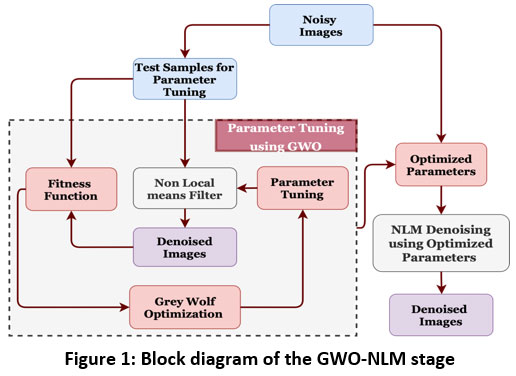Figure 1: Block diagram of the GWO-NLM stage Click here to view Figure

Local Means Filters find the pixels average value around the neighborhood of a target pixel, then replace target pixel with those values. Though this operation smoothens the image by removing odd pixels, it may also introduce an undesired blurring effect near the edges. On the other side, the non-local means filtering algorithm considers a nearby area around the target pixel and then finds the identical patches in that particular search space and replaces the center pixel with a weighted average with respect to selected patches center pixels. Each patch is assigned a weight depending on its similarity to the target patch. Thus, in NLM filtering, the updated pixel value mostly depends on the center pixels of the patches very close to the target patch and can retain the relevant details such as edges and corners.

The GWO algorithm is designed to simulate the natural leadership mechanism in hierarchical and hunting fashion of grey wolves. Based on the ranking, a wolf pack can be divided into four categories namely alpha (α), beta (β), delta (δ), and omega (ω). Here, Alpha is leader of the wolves during hunting, alpha, beta, and delta wolves altogether adjust and modify their locations in response to the prey’s position, while omega wolves follow either of them. The GWO model treats alpha, beta, and delta wolves as primary search agents, with their positions as the optimal solutions to the optimization problem given. The search agent’s locations are updated with respect to the fitness function. Hence, Once the fitness function starts converging and obtain optimal value, the average of the alpha, beta, and delta wolves search agent last locations will be considered as the optimal solution.

In the proposed denoising algorithm, the patch size () around each target pixel, research window radius (), and filtering parameter () control the degree of smoothing and is planned to adjust it adaptively based on an optimal trade-off between the degree of filtering and the time complexity to process the image. Therefore, the search agent space will be in 3D space represented using ,  and . These parameters are updated in each iteration and hence an   search agent () at  iteration can be represented as . The number of search agents is also critical while designing a GWO model.

The GWO algorithm initializes with a set of random values of the search agent parameters and will pass through the fitness function:

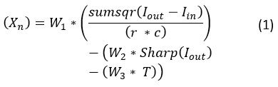
where  is the output of the NLM filter with input image ,  indicates the sharpness of the image,  and  are the rows and columns in the image, , , and  are the weights used to assign a balance between various criteria, and  represent the time complexity in seconds while filtering the image.

The following steps describe the various stages in a GWO-NLM denoising approach.

Step 1: Initialization of the search agents.

The no. of search agents corresponds to the number of wolves in the pack. So, there can be a minimum three search agents (alpha, beta, and delta). The higher the search agents, more omega wolves will be in action that leads to a better optimization at the cost of computational cost being increased.

Let X is the group of searches agents’ elements, where Xⁿ represents the position of search agent. The representation of the search agent location is mainly depending on the no. of parameters required to obtain optimized solution for a given problem. The proposed algorithm uses five search agents which is analogous to a pack of five wolves. During initialization, the search agent’s initial positions are always initialized with some random values within the parameter’s lower and upper bounds. ,  and  parameters are optimized in the case of NLM optimization, and the equation will be

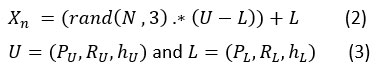
where (P_U,R_U,h_U) and (P_L,R_L,h_L) denotes upper bound , lower bound of patch size, search radius, and degree of filtering. 

Step 2: Finding alpha, beta and delta search agents.

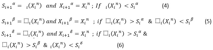
Compute the objective function Δ_i(X_n ) corresponding to each search agent based on their values at  iteration. This will be calculated for all search agents, and the scores of alpha, beta and delta search agents are updated based on this fitness values as shown below.

Let X_iⁿ; n={1,2,…, N} is the set of search agents, X_i ^α , X_i ^β , X_i ^δ and  are the positions of alpha, beta and delta search agents, and S_i ^α , S_i ^β , S_i ^δ and are the fitness scores of alpha, beta and delta in the i^th iteration, their values are updated as shown below.

Step 3: Update the remaining search agents positions.

After updating the high ranked alpha, beta, and delta agents based on the fitness function, the remaining search agents are also updated with respect to the positions of these alpha, beta, and delta agents. Mathematically, they are shown in following equations.

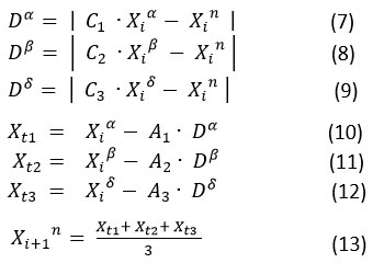
where the constant vectors C₁, C₁,C₃  and A₁, A₁, A₃  are computed by using the formula

and r₁ , r₂ and  are the random vectors in the range [0, 1] and  is linearly decaying from 2 to 0.

Hence the locations of alpha, beta, and delta is directly depending on the fitness values and the omega search agents are based on the average positions of those top three search agents.

Step 4: Stopping criteria.

Steps 2 and 3 are repeated iteratively to update the positional vectors of the search agents in order to arrive at the optimal condition. Because the entire process is iterative, a stopping criterion is required to terminate the process once it reaches an optimal state. As a result, a stopping criterion is defined based on Fitness value or specifying a fixed number of executed iterations.

Image Normalization

The denoised image is planned to process via a CNN model and converted to a Z-normalized form to reduce the redundancy in the data and make it in a finite range of 0 – 1. It is achieved by subtracting the mean value from the data and dividing it using the standard deviation.

Semantic Segmentation

The proposed method uses a deep learning architecture that uses an encoder-decoder based Convolutional neural network model with several optimization modules. The approach uses attention modules, residual connections, and rigorous supervision to improve learning. The U-Net architecture with a depth of 4 is used as the baseline architecture. The encoding and decoding stages include a combination of traditional convolution layers and residual modules. By customizing the network architecture, Our proposed implemented model overcomes several shortcomings of the mainstream CNN based segmentation architectures. The following sections provide an in-depth explanation of the proposed segmentation model.

Figure 2: Block diagram of the Proposed Segmentation network. Click here to view Figure

CNN Architecture

The proposed model uses a series of normal convolution layers and residual convolution blocks in each encoder and decoder depths to leverage multiscale feature extraction and reduce computation cost. A standard convolution layer is used in each depth, followed by a residual block consisting of two standard convolution layers. This will contribute a total of three successive convolution operations with 3×3 kernels and lead to a feature extraction at three different scales (3×3, 5×5, and 7×7). The identity mappings in the residual block reduce the feature degradation problem and vanishing gradient issues and improve learning performance by enabling better convergence through several possible network paths.

Another advantage of these residual connections is in reducing the computational overhead. When the number of convolution layers increases, the computation cost often increases significantly due to the quadratic effect [16]. in the increase in parameters. This will contribute considerable multiplications and lead to an undesirable training time complexity. Furthermore, the quadratic effect increases the memory required to process additional feature space. Hence, spreading the trainable parameters into multiple convolution layers per depth using residual blocks helps promote better learning with less computation complexity.

The proposed network architecture uses a module called attention gates to regulate the pass of finer features in both the encoder and the decoder frameworks. Oktay et al. [17] proposed one of the first deep learning system for segmentation using an attention gated U-Net model. Attention modules aid in guiding the learning by focusing more on the relevant areas of the image where significant characteristics are located. Though pooling operations in the standard U-Net architecture’s encoder stage helps pass relevant features to the deeper layer, it also causes the loss of finer details due to the down sampling of feature spaces. This lack of learning about the finer features may reduce saliency and affect segmentation efficiency, and skip connections are usually preferred in FCNN frameworks to reduce these issues.

However, long skip connections cannot preserve the saliency in the layers in advanced depths and may lead to a semantic disparity between the encoder and decoder features. In addition, as the activation outcomes at deeper layers have a greater level of detail, using the attention modules in advanced depths aids in negating irrelevant features and passing salient information from the field of interest of the image. The proposed segmentation network utilizes a convolutional block attention module (CBAM) [18] comprised of a channel and a spatial submodule, where they highlight the prominent features through a set of parallel convolutional processes.

The model also uses residual blocks to pass features from encoder to decoder path at shallow depths. This will minimize the semantic gap between the activation outcomes of the starting and ending layers and makes the feature concatenation more useful. In order to preserve the high-level features at the advanced encoder layers and to minimize the semantic gap between the shallow depths, the initial depths (depth-0 and depth-1) uses more residual blocks in the skip connection, depth-2 and depth-3 use a single residual block to bypass the features, and the depth-4 uses an attention block.

The side layers in figure 2 illustrate the “deep supervision” [19], in which the final classification layer uses upsampled activation from all decoder levels after appropriately resizing the feature map via transpose convolution. Hence, the final classification layer can directly assess on features from various image scales and contributes comprehensive learning in the network. 

Training Methodology

Each convolutional layer in the encoding path (both standard convolution and residual block) utilizes batch normalization and ReLU activation [20]. The proposed model employs a depth-3 CNN architecture and operates on 512×512 image resolution. All convolutions use 32 kernels in depths 0 and 1, and the no. of kernels increases in successive layers. As a result, the depth-2 and depth-3 encoder stages employ 64 and 96 kernels, respectively. The hyperparameters such as the number of kernels in each layer, the no. of layers in the residual block, and network depth are designed based on the feedback obtained from several experiments. The increasing number of kernels in the higher depths helps widen the feature space and compensate for the feature size reduction due to max-pooling. Through the CBAM activation module, the bottleneck features are passed from the last encoding layer to the foremost decoding layer. Besides, CBAM is integrated prior to the final classification layer in order to concentrate the characteristics primarily from the region of interest.

The decoding path employs appropriate reverse operations to increase the resolution of the feature space to that input image. The Transposed convolution is used to perform the up sampling. The encoding path’s feature maps are concatenated with the decoding layers via skip connections. Additionally, L2 regularizes [21] are included to prevent overfitting. The final classification layer employs the sigmoid activation function to scale the segmentation map’s probability values into the range [0,1].

The loss function is another parameter that can significantly impact while updating the trainable weight parameters. Our model, aims at segmenting the bone regions from X-ray images and hence the chance of class imbalance between the foreground class (bone region) and background class (soft tissue region + image background). This particular class imbalance can affect the required learning process and adversely affect the segmentation performance. Hence, the current work uses a loss function Tversky loss function [22] that can handle the bias in the segmentation classes. While using the Tversky loss function, the weighing factors for false negatives and false positives can be adjusted and considered a generalized Dice loss. This enables the model to train by keeping a good precision-recall trade-off based on the input data. Mathematically, the Tversky loss function is depicted as:

where TP, FP , FN and  represents false positive, true positive and false negative and α and β are the weight factors. The values of α and β are chosen as 0.2 and 0.8 experimentally, based on the performance of the bone segmentation dataset in both recall and precision evaluation.

We performed 5-fold cross-validation method to avoid bias and statistical related uncertainty. In each fold, the entire data has been split into training data and testing data in an 80:20 ratio. 20% of the training data is again considered as the validation data and is mainly used to save the weight parameters during the training process. A starting learning rate of 0.001 with the Ad grad optimizer [23] is used while updating the kernel weights. For weight initialization, He normal weight initialization is used, and the training was performed with a batch size of 8. As the no. of samples in the bone segmentation dataset is less, an online augmentation is also performed. Flip, Rotation, and sheer augmentation is been performed for increasing the no. of training samples. Our model has also been trained up to 100 epochs by keeping an early stopping patience of 50 epochs

Results and discussion

Dataset

The study uses XSITRAY [24] dataset that consist of 48 high resolution unannotated X-ray images. It consists of X-ray scans of various body parts including chest, femur, ankle, elbow etc. The dataset images are resized to a standard resolution of 512×512 pixel resolution and are manually annotated with the supervision of expert medical practitioners.

Experimental Setup

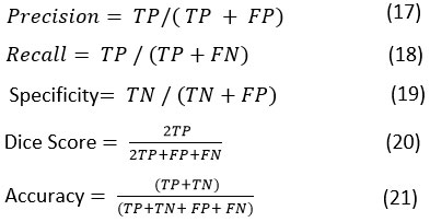
Analysis and comparison of our proposed model’s performance with other similar models have been carried out both quantitatively and qualitatively. All experiments were carried out using Python programming with the Keras library. Google Colab is used to implement the model and to perform an ablation study for finetuning the hyperparameters. Precision, specificity, recall, Dice score, and accuracy are the segmentation benchmarks used to demonstrate the performance of the model from various perspectives in this quantitative analysis. Mathematical representations of these benchmarks are depicted below.

The quantitative results shown in Table 1 are obtained by comparing the proposed segmentation technique to a state-of-the-art model with the same dataset.

Figure 3: Training performance of proposed model for 100 epochs. Click here to view Figure

The model performance in updating the loss values is shown in figure 3. The testing loss almost follows the training loss pattern and shows a right fitted model for the target bone segmentation.

The results obtained from the proposed segmentation model are analyzed quantitatively and are illustrated in Table 1. It has been analyzed and compared with a state-of-the-art bone segmentation model to show its superiority in extracting bone regions. While implementing the existing model, we have used the same X-ray dataset and trained from scratch for a fair comparison. To validate the effectiveness of the design aspects of the proposed model, the analysis also includes an ablation study with various design elements.

Table 1: Quantitative analysis to assess the segmentation performance

Method	Precision	Recall	Dice Score	Specificity	Accuracy
Fathima	75.17	90.60	82.16	83.79	86.18
Proposed method (without denoising)	86.69	76.08	81.04	93.67	87.50
Proposed method (with Shock filter)	88.77	81.25	84.84	94.42	89.80
Proposed method (with GWO-NLM)	85.82	88.36	87.07	92.1	90.79

The quantitative analysis Table 1. Demonstrates a significant improvement when the proposed model is used. The model is constrained by severe data issues such as limited training samples and inter-class similarity between the bone and soft tissue regions. These limitations are overcome by incorporating several design elements that enhance the overall segmentation performance. The performance of the proposed model with numerous ablations also exemplifies the effectiveness of the suggested denoising step in proficiently extracting the bone regions.

In biomedical image analysis like bone segmentation, precision and recall are highly significant to keep a better output without missed regions or over-segmented false detections. Since the Dice score represents the recall and harmonic mean of precision, its higher values point to a better segmentation that evaluates the similarity of the prediction map with respect to the actual ground truth image. In the ablation study, we used the proposed CNN in three combinations: without pre-processing, shock filter-based denoising, and GWO-NLM denoising. In the proposed method with GWO-NLM, the precision and recall are high and have the highest Dice score compared with the state-of-the-art CNN model for bone segmentation. The proposed segmentation model shows the best precision performance with the shock filter but with undesired recall results. Overall results with the model without denoising also show inferior results compared to other ablations.

Segmentation outcomes are also evaluated qualitatively by visually examining the test samples, and a few randomly selected test samples are shown in figure 4. The obtained results show the advantage of the proposed model against other approaches, especially in avoiding the missing bone pixels without adding too many false positives.

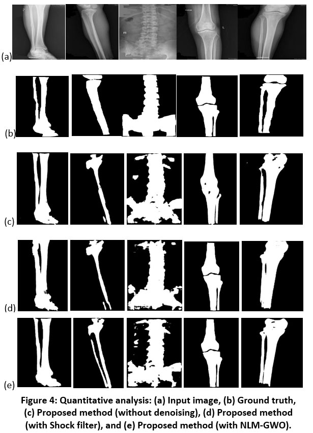Figure 4: Quantitative analysis: (a) Input image, (b) Ground truth, (c) Proposed method (without denoising), (d) Proposed method (with Shock filter), and (e) Proposed method (with NLM-GWO). Click here to view Figure

Conclusion

The current study focused on solving a bone segmentation problem from X-ray images. Our proposed model uses an exclusive denoising algorithm that uses a GWO optimization with an NLM filter for adaptively estimating the denoising parameters. This helped avoid manual finetuning and saved much time in batch pre-processing. The proposed segmentation model uses a complex CNN module that uses various modules such as attention gates, residual blocks, and deep supervision that helps to solve several drawbacks of the standard U-Net model to extract information from small datasets. The learning uses custom loss function: Tversky loss to give proper weightage to both the precision and recall and hence improving the overall segmentation performance.

Conflict of Interest

There is no conflict of interest.

Funding Sources

There are no funding sources.

References

1. J Kasban H, El-Bendary MA, Salama DH. A comparative study of medical imaging techniques. International Journal of Information Science and Intelligent System. 2015 Apr;4(2):37-58.
2. Raza K, Singh NK. A tour of unsupervised deep learning for medical image analysis. Current Medical Imaging. 2021 Sep 1;17(9):1059-77.
   CrossRef
3. Ker J, Wang L, Rao J, Lim T. Deep learning applications in medical image analysis. Ieee Access. 2017 Dec 29;6:9375-89.
   CrossRef
4. Ronneberger O, Fischer P, Brox T. U-net: Convolutional networks for biomedical image segmentation. InInternational Conference on Medical image computing and computer-assisted intervention 2015 Oct 5 (pp. 234-241). Springer, Cham.
   CrossRef
5. Stolojescu-Crisan C, Holban S. An Interactive X-Ray Image Segmentation Technique for Bone Extraction. InIWBBIO 2014 (pp. 1164-1171).
6. Umadevi N, Geethalakshmi SN. Enhanced Segmentation Method for bone structure and diaphysis extraction from x-ray images. International Journal of Computer Applications. 2012 Jan;37(3):30-6.
   CrossRef
7. El-Feghi I, Huang S, Sid-Ahmed MA, Ahmadi M. X-ray image segmentation using auto adaptive fuzzy index measure. InThe 2004 47th Midwest Symposium on Circuits and Systems, 2004. MWSCAS’04. 2004 Jul 25 (Vol. 3, pp. iii-499). IEEE.
8. Ding L, Zhao K, Zhang X, Wang X, Zhang J. A lightweight U-Net architecture multi-scale convolutional network for pediatric hand bone segmentation in X-ray image. IEEE Access. 2019 May 22;7:68436-45.
   CrossRef
9. Bullock J, Cuesta-Lázaro C, Quera-Bofarull A. XNet: A convolutional neural network (CNN) implementation for medical X-ray image segmentation suitable for small datasets. InMedical Imaging 2019: Biomedical Applications in Molecular, Structural, and Functional Imaging 2019 Mar 15 (Vol. 10953, p. 109531Z). International Society for Optics and Photonics.
   CrossRef
10. Shen W, Xu W, Zhang H, Sun Z, Ma J, Ma X, Zhou S, Guo S, Wang Y. Automatic segmentation of the femur and tibia bones from X-ray images based on pure dilated residual U-Net. Inverse Problems & Imaging. 2021;15(6):1333.
    CrossRef
11. Nazia Fathima SM, Tamilselvi R, Parisa Beham M, Sabarinathan D. Diagnosis of osteoporosis using modified U-net architecture with attention unit in DEXA and X-ray images. Journal of X-Ray Science and Technology. 2020(Preprint):1-21.
    CrossRef
12. Nazia Fathima SM, Tamilselvi R, Parisa Beham M, Sabarinathan D. Diagnosis of osteoporosis using modified U-net architecture with attention unit in DEXA and X-ray images. Journal of X-Ray Science and Technology. 2020(Preprint):1-21.
    CrossRef
13. Manson EN, Ampoh VA, Fiagbedzi E, Amuasi JH, Flether JJ, Schandorf C. Image Noise in Radiography and Tomography: Causes, Effects and Reduction Techniques. Current Trends in Clinical & Medical Imaging. 2019;2(5):555620.
14. A Buades A, Coll B, Morel JM. A non-local algorithm for image denoising. In2005 IEEE Computer Society Conference on Computer Vision and Pattern Recognition (CVPR’05) 2005 Jun 20 (Vol. 2, pp. 60-65). IEEE.
15. Mirjalili, Seyedali, Seyed Mohammad Mirjalili, and Andrew Lewis. “Grey wolf optimizer.” Advances in engineering software69 (2014): 46-61.
16. Niyas S, Vaisali SC, Show I, Chandrika TG, Vinayagamani S, Kesavadas C, Rajan J. Segmentation of focal cortical dysplasia lesions from magnetic resonance images using 3D convolutional neural networks. Biomedical Signal Processing and Control. 2021 Sep 1;70:102951.
    CrossRef
17. Oktay O, Schlemper J, Folgoc LL, Lee M, Heinrich M, Misawa K, Mori K, McDonagh S, Hammerla NY, Kainz B, Glocker B. Attention u-net: Learning where to look for the pancreas. arXiv preprint arXiv:1804.03999. 2018 Apr 11.
18. Woo S, Park J, Lee JY, Kweon IS. Cbam: Convolutional block attention module. InProceedings of the European conference on computer vision (ECCV) 2018 (pp. 3-19).
    CrossRef
19. Wang L, Lee CY, Tu Z, Lazebnik S. Training deeper convolutional networks with deep supervision. arXiv preprint arXiv:1505.02496. 2015 May 11.
20. Agarap AF. Deep learning using rectified linear units (relu). arXiv preprint arXiv:1803.08375. 2018 Mar 22.
21. Cortes C, Mohri M, Rostamizadeh A. L2 regularization for learning kernels. arXiv preprint arXiv:1205.2653. 2012 May 9.
22. Salehi SS, Erdogmus D, Gholipour A. Tversky loss function for image segmentation using 3D fully convolutional deep networks. InInternational workshop on machine learning in medical imaging 2017 Sep 10 (pp. 379-387). Springer, Cham.
    CrossRef
23. Duchi J, Hazan E, Singer Y. Adaptive subgradient methods for online learning and stochastic optimization. Journal of machine learning research. 2011 Jul 1;12(7).athima SN, Tamilselvi R, Beham MP. XSITRAY: a database for the detection of osteoporosis condition. Biomedical and Pharmacology Journal. 2019 Mar 25;12(1):
24. CrossRef
25. Dodamani, Pooja S., and Ajit Danti. “Assesment of Bone Mineral Density in X-ray Images using Image Processing.” 2021 8th International Conference on Computing for Sustainable Global Development (INDIACom). IEEE, 2021.

(Visited 256 times, 1 visits today)