Neelam Turk^1*, Sangeeta Kamboj² , Sonam Khera¹ and Neha Rajput¹

¹Electronics and Communication Engineering Department, J.C.Bose  University of Science and Technology, YMCA ,Faridabad, Haryana, India. 121006.

²Electrical and Instrumentation Engineering Department, Thapar Institute of Engineering and Technology, Patiala, Punjab, India. 147001

Corresponding Author E-mail: engineersangeeta@gmail.com

DOI : https://dx.doi.org/10.13005/bpj/2188

Abstract

In the proposed work, noise models such as Salt & Pepper, Gaussian and Poisson are considered in order to corrupt the image.Image restoration is still challenging task to recover an original  image using a degradation and restoration model. In the paper, Gaussian, Average and Wiener linear image restoration techniques are used to recover the original MRI image. Median filter, Min and Max non-linear filters are also used to obtain uncorrupt image in the paper.Mean square error (MSE), Peak Signal to Noise Ratio (PSNR) and Cross Correlation(CC) performance analysis criteria are used to compare different restoration technique so that better performance in a clinical diagnosis can be achieved. In the paper it can be found that wiener filter with 5 x 5 window for Gaussian, speckle and Poisson noise provides best performance in terms of MSE and PSNR. Also,median filter with 5 x 5 window gives better accuracy of results to restore 3D salt & pepper noised image in terms of MSE and CC.

Keywords

Image degradation; Image restoration; Linear and Nonlinear filter; MRI image; MSE; PSNR

Download this article as: 

Copy the following to cite this article: Turk N, Kamboj S, Khera S, Rajput N. Performance Analysis of Different Restoration Techniques for Degraded 3d Cervical Spine Mri Image. Biomed Pharmacol J 2021;14(2).

Copy the following to cite this URL: Turk N, Kamboj S, Khera S, Rajput N. Performance Analysis of Different Restoration Techniques for Degraded 3d Cervical Spine Mri Image. Biomed Pharmacol J 2021;14(2). Available from: https://bit.ly/3ywGIrI

Introduction

The Image processing takes an image as an  input and provides uncorrupted output image or original image information. In the present scenario, digital image processing is used in various fields such as medical imaging processing for diagnosis of diseases, face recognition for security purposes and resource exploration[1]. There are several degradation sources such as noise and blur presented in the available literature which may corrupt the image[2,5,7,8,12]. The process of recovering an image that has been degraded by a son degradation process is known as Image Restoration. In the field of engineering, digital image processing introduced a different kind of image restoration methods to recover original scene from degraded observations. The noise removal method should be applied in accurate manner in order to obtain precise image in medical image processing [2]. Various restoration techniques Image restoration techniques exist both in spatial and frequency domain. In the proposed work, motion, out of focus and environmental turbulence blurs are considered in degradation of 3D cervical spine MRI Image. In the paper Salt and Pepper, Gaussian, Speckle and Poisson noises are added in order to corrupt image. The linear (Gaussian filter. Average filter, Poisson filter) and nonlinear (Median, Minand Maxfilter) restoration techniques both are used to obtain preciseimage so that uncorrupted image can be used to get correct observations for the given application in medical image process. In the paper, MSE, PSNR and CC performance analysis criterions are used for selection of best filter for a particular type of noise model to recover noiselessly and deblurred image and thus to enhance performance of restoration techniques.

Image Degradation Models

Image acquisition depends on the quality of sensing elements, transmission media and environmental conditions such as atmospheric disturbance, humidity, light, and temperature etc. In the proposed work, degradation of image is also done by motion blur, out-of-focus and environmental turbulence blurs. Motion blur is the visible line of a different colour of moving objects [3]. It is the most widely recognized corruption types found in the customer photography. In most cases, the out of focus blur caused by a system with a circular aperture. An Image formed by connecting the stage of optical system analogous to a lens, selected depth of the object is aimed by the lens, but the objects at different distances are corrupted by different level calculating on their distances. The parameters on which the camera focus depends on focal distance, wavelength of  the incoming light object, object depth and aperture size [4]. This type of Long-term exposure to atmospheric distortions is commonly experienced in remote sensing and aerial imaging caused by optical turbulence and scattering and absorption by particulate results in a degraded image [3]. Salt and Pepper, Gaussian, Speckle and Poisson which are added in order to corrupt 3D cervical spinal MRI image and described as follows:

Salt & Pepper Noise or Impulse Noise

This noise appears in images as black and/or white impulse of the image. The noise is due to  white and black spots which chaotically scattered gray scale images along image area. The Power Density Function for Salt & Pepper noise is given as ^5,12 :

The basic steps which are used to add salt and pepper noise into RGB and Gray Scale imageare given as:

First color image is converted into monochrome image.

Random values will be generated by “randn” function for the given matrix size within the specified range. Consider an image matrix of size 4×3 image matrix as:

4	10	4
7	8	4
10	0	5
3	10	9

The random matrix 4x3is generated with range 0 to 10. Let random   matrix be:

237	107	166
234	95	162
239	116	169
56	126	89

If there is ‘0’ value in the random matrix this pixel value is now replacing with zero or black. After that, black pixel is entered in image matrix.

237	107	166
234	95	162
239	0	169
56	126	89

Similarly image matrix contains white pixel by replacing pixel value ten with pixel value 255 if random matrix contains pixel value 10. Finally, the image matrix become,

237	255	166
234	95	162
255	0	169
56	126	89

The effect of the addition of this noise in RGB and Gray Scale Image is shown in Figure 1.

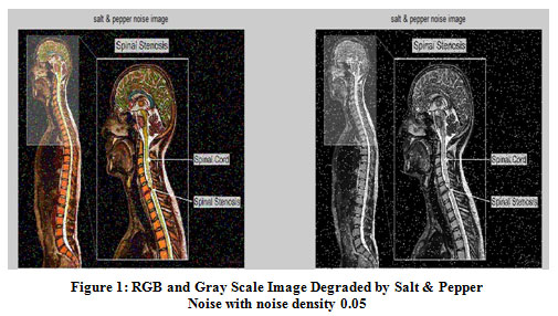Figure 1: RGB and Gray Scale Image Degraded by Salt & Pepper Noise with noise density 0.05 Click here to view figure

Gaussian Noise

Gaussian noise is one of the most occurring noise and also called additive noise. In this noise certain distribution is added to each pixel in order to modify it [2,12]. Whenever this noise appears, then receiver interprets received sample value y(k) at the kth sample time as the sum of noise-free component y₀(k), i.e., the sample value that would have been received at the kth sample time in the absence of noise and  noise component w(k), assumed independent of the input waveform. It can be written as:

The noise component w(k) is irregular, but assumed to be drawn at each sample time from a fixed Gaussian distribution for concreteness. And RGB and Gray Scale Image which is degraded by Gaussian Noise with noise variance 0.005 is presented in figure 2.

Figure 2:  RGB and Gray Scale Image Degraded by Gaussian Noise with noise variance 0.005 Click here to view figure

Speckle Noise

This noise is usually modeled by random element multiplication with pixel elements of the image [6]. The random settlement of the pixel in the image appears due to inherent characteristic of ultrasound imaging. This unknown settlement of the pixel in the image is known as speckle noise. Radical reduction in distinction resolution due to speckle noise produces a  negative impact on medical imaging [7]. The speckle noise can be modelled as:

Where, h(n,m) is the observed image, u(n,m) is the multiplicative component and 𝜂(n,m) is the additive component of the speckle noise. Here n and m denote the axial and lateral indices of the image samples. For the ultrasound imaging, an only multiplicative component of the noise is to be considered and additive component of the noise is to be ignored. Hence, equation (1) can be modified as;

The behavior of Speckle pattern depends on the number of disperse per resolution cell or disperse number density. In the figure 3, speckle noise with noise density 0.04 is added to RGB and Gray Scale Image to degrade it.

Figure 3: RGB and Gray Scale Image Degraded by Speckle Noise with noise density 0.04. Click here to view figure

Poisson Noise

When the electromagnetic waves of high energy are injected into patient’s body from its source, this noise appears due to the statistical nature of electromagnetic waves on medical instrument of imaging systems. The noise is also called as quanta (photon) noise or shot noise. This noise obeys the Poisson distribution which is given as :

Where λ is the expected number of the particles i.e. photons per unit time interval, which is proportional to the occurrence of the scene radiance. A rate parameter ‘𝜆𝑡’ is known as the standard Poisson scattering or distribution which corresponds to the expected incident photon count. The uncertainty described by this diffusion is known as photon noise. Photon noise include random electron emission which consists of Poisson distribution with mean square value [8].Because the occurrence of the light particle count follows a Poisson scattering, it has the property that its variance is equal to its expectation that is  represented by equation 4.

This shows that its standard deviation grows with the square root of the signal and photon noise is information or signal dependent. Photon noise variance depends on the expected photon count and is often modelled using a Gaussian distribution as:

This approximation in most cases is very accurate. According to the central limit theorem, for larger particles of light count or photon count Poisson distribution approaches to Gaussian distribution and for the small particles of  light counts  photon distribution is dominated by other signal independent sources of random signal.The effect of Poisson noise after its addition in RGB and Gray Scale Image is presented in figure 4.

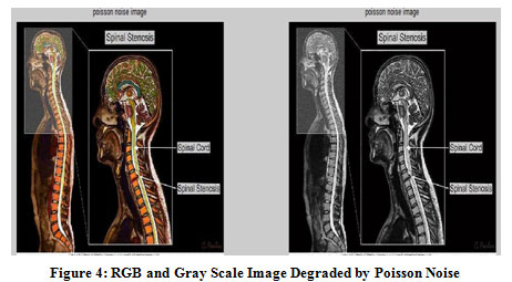Figure 4: RGB and Gray Scale Image Degraded by Poisson Noise. Click here to view figure

Image Restoration Techniques

Linear Restoration Method

In this method the original image is to be convolved with a mask. The mask represents a low-pass filter or smoothing operation which is used to restore certain type of noised images. The output of a linear operation due to the sum of two inputs is same as that of performing the operation on the inputs individually and then summing the results.Some of the linear restoration methods used to restore the captures 3D MRI image are given as:

Gaussian Filter

It works by using the 2D distribution as a point-spread function. This is achieved by convolving the 2D Gaussian distribution function with the image. And to implement it steps which are used are given as:

Design the kernel window.

Use formula to design 2D Gaussian kernel.

For this consider the standard deviation, sigma =0.6 and the kernel size 3×3. i.e

(1/2𝜋𝜎²) = 1/2.2619

The width of the kernel is X=3 and the height of the kernel is Y=3.

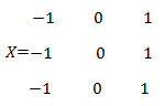
and

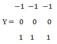
The Gaussian kernel’s dominant part (Here 0 .4421)has the highest value and intensity of other element decreases the distance from the median or dominant part increases. Now the Gaussian kernel is:

0.0275	0.1102	0.0275
0.1102	0.4421	0.1102
0.0275	0.1102	0.0275

Convolve the kernel and the local region from an image

72	68	88	159
69	66	87	162
70	66	83	161
70	66	78	154

Convolve the selected part and the kernel

68	88	159		0.0275	0.1102	0.0275		1.8692	9.7009	4.3706
66	87	162	.∗	0.1102	0.4421	0.1102	=	7.2757	38.4624	17.8585
66	83	161		0.0275	0.1102	0.0275		1.8142	9.1497	4.4256

Add up the values in the vector: – 1.8692 + 9.7009 + 4.3706 + 7.2757 + 38.4624 + 17.8585 +1.8142 + 9.1497 + 4.4656 = 94.9269

On convolution of the local region and the Gaussian kernel gives the highest intensity value to the center part of the local region(38.4624)and the remaining pixels have less intensity as the distance from the center increases.The result obtained from the total sum is stored in the present pixel location (Intensity=94.9269) of the image.

[]	[]	[]	[]
[]	[]	94.9269	[]
[]	[]	[]	[]
[]	[]	[]	[]

Average Filter

The filter operates on a m x n mask by taking average of all pixel values within the window and replace the center pixel value in the final image with the result. It also causes a certain amount of blurring in the image ¹¹.

Let 𝑓_𝑖𝑗, for i, j = 1,…,n, denote the pixel values in the image. Here  g is used with  pixel values 𝑔_𝑖𝑗, to denote the output from the filter. A linear filter of size (2m+1)×(2m+1), with specified weight 𝑤𝑘𝑙for k, l =  – m, . . . , m, gives :

𝑓𝑜𝑟𝑖,𝑗=(𝑚+1)………,(𝑛−𝑚)

For example, if m = 1, then the window over which averaging is carried out is 3 × 3, and

𝑤−1,−1𝑓𝑖−1,𝑗−1	+𝑤−1,0𝑓𝑖−1,𝑗	+𝑤−1,1𝑓𝑖−1,𝑗+1
+𝑤0,−1𝑓𝑖,𝑗−1	+𝑤0,0𝑓𝑖,𝑗	+𝑤0,1𝑓𝑖,𝑗+1
+𝑤1,−1𝑓𝑖+1,𝑗−1	+𝑤1,0𝑓𝑖+1,𝑗	+𝑤1,1𝑓𝑖+1,𝑗+1

The weights (w) can depend on i and j for full generality and result in a filter which vary across the image. Also, all the filters will have windows composed of odd numbers of rows and columns. It is possible to have even-sized windows, but there will be half-pixel displacement between the input and output images.

Wiener Filter

It is a digital filter used to adjust variable parameters obtained due to mathematical programming. This filter is applied to the degraded image to adjust the local variance of the image. By adjusting its variance means calculating the distance between random number or noisy pixel and average of those pixels centered within the mask. Smoothing of the image is totally depending upon the variance of the image. Large value of the variance results in less smoothing and small value of the variance results in more smoothing. This type of linear filtering is more adaptive in the field of image processing as it produces better results. The following steps are used for its implementation:

Define a window of size m x n

Consider matrix B with Gaussian noise.

	0.9361	1.000	1.000	0.8871
B=	1.000	1.000	0.9184	1.000
	0.9868	1.000	1.000	0.9591
	0.000	0.8987	0.9400	1.000

Let window size be 3×3 and pad the matrix B with zeros on allsides.

48.7478	59.2645	79.7865	100.2444
57.1176	69.7512	94.9269	121.1870
57.1740	68.9526	92.2220	119.6981
47.7534	59.9750	74.1254	96.7113

 

0	0	0	0	0	0
0	0.9361	1.000	1.000	0.8871	0
0	1.000	1.000	0.9184	1.000	0
0	0.9868	1.000	1.000	0.9591	0
0	0.000	0.8987	0.9400	1.000	0
0	0	0	0	0	0

Compute the local mean and local variance by sliding the 3×3 window

0	0	0
window=0	0.9361	1.000
0	1.000	1.000

Local mean=mean (window) =0.4373 Local variance = mean (window²) – mean (window) ² = 0.2394

Then local mean matrix for the given matrix B

0.4373	0.6505	0.6451	0.4228
0.6581	0.9824	0.9738	0.6405
0.5428	0.8604	0.9685	0.6464
0.3206	0.5362	0.6442	0.4332

The local variance for the given matrix B is:

0.2394	0.2124	0.2095	0.2246
0.2169	0.009	0.0017	0.2064
0.2366	0.0939	0.0015	0.2096
0.2063	0.2309	0.2085	0.2349

The variance of the overall noise is the average of the local variance Hence, variance of noise=0.1709.If (noise variance > local variance (x,y)) then Local variance (x,y)=noise variance Here,(x,y) represent the pixel positions in two dimension finally, local variance becomes:

0.2394	0.2124	0.2095	0.2246
0.2169	0.1709	0.1709	0.2064
0.2366	0.1709	0.1709	0.2096
0.2063	0.2309	0.2085	0.2349

Final image = B – (noise variance / local variance) (B – local mean)

0.5802	0.7188	0.7105	0.5339
0.7307	0.9824	0.9738	0.7025
0.6662	0.8604	0.9685	0.7042
0.2656	0.6304	0.6975	0.5878

Nonlinear Restoration Method

In this method, it is necessary to impose constraints such as non-negativity i.e. either positive or zero to implement spatial adaptively and recover missing spatial or frequency components at the expense of economical implementation and native convergence.  Non-linear filters preserve the details of the image. Non-linear filters have many applications, especially removal of noise that is not additive [10]. Some of the nonlinear restoration methods used in the proposed work are given as:

Median Filter

It is one of the order Statisticor Rank Filter due to its nature of edge preserving. In this middle pixel value from the ordered set of values with in the mxn neighborhood(W) around the reference pixel is selected[2,4]

And an output value of pixel is determined by replacing the value of each corresponding pixel by the median of the neighboring pixels, rather than the mean. The mean of the extreme values of the pixels in the degraded image is more sensitive to its median. This filter has ability to preserve the edges of the image i.e contrast or sharpness of image. The image filtered with 3×3 windows still contains salt and pepper noise, but the edges are sharp.The image filtered with a larger window size contains less noise as compared to less window size. Now the implementation process used to restore the corrupted image is given as:

Let the original image with the matrix

4	6	9
2	5	3
8	1	7

Now apply paddingon the image matrix

0	0	0	0	0
0	4	6	9	0
0	2	5	3	0
0	8	1	7	0
0	0	0	0	0

Consider a mask of size 3 by 3. Them ask can be of any size. Starting from matrix A(1,1) and place the window

0	0	0
𝑤𝑖𝑛𝑑𝑜𝑤=0	4	6
0	2	5

The middle pixel value A (2, 2)will be change after sorting

0	0	0
𝑤𝑖𝑛𝑑𝑜𝑤=0	4	6
0	2	5

After Sorting the mask matrix. Now the new matrix is

0	0	0
0	0	2
4	5	6

The pixel value of the out put image matrix is replaced by median 0. The value of the output pixel is found using the median of the neighboring pixels.Repeat this process until the whole matrix is replaced by the median values after that the final output matrix is

0	3	0
2	5	2
0	2	0

Min and max filter

It works on a ranked set of pixel values. Them in filter, also known as the zero thpercentile. The min filter replaces there ference pixel with the lowest value [11]. Similarly,the max filter,also known as the 100 thpercentile filter, replaces the reference pixel within the window with the highest value. Now the following steps are used for the implementation of max filter to recover the original image:

Consider matrix A

1	2	2	1
1	1	0	3
2	4	1	5
2	1	2	0

Pad matrix with zeros and matrix A will be:

0	0	0	0	0	0
0	1	2	2	1	0
0	1	1	0	3	0
0	2	4	1	5	0
0	2	1	2	0	0
0	0	0	0	0	0

Consider the elements in the window 3 x 3

0	0	0	0	0	0
0	1	2	2	1	0
0	1	1	0	3	0
0	2	4	1	5	0
0	2	1	2	0	0
0	0	0	0	0	0

i.e

1	2	2
1	1	0
2	4	1

Find the maximum from the window. Here it is 4.Similarly, find the maximum by sliding the window on the whole matrix.Thus output matrix becomes:

2	2	3	3
4	4	5	5
4	4	5	5
4	4	5	5

Similarly the following steps can be used to implement min filter:

Find the darkest points in an image.

Also find the minimum value in the area encompassed by the filter.

Reduces the salt noise as a result of the min operation.

The 0 thpercentile filter is min filter.

Results and Discussion

Image restoration techniques as discussed in section 3 has been applied to degraded 3D cervical spine MRI image to improve denoising of the  image. In the figures 5- 10, input image is corrupted using Salt &Pepper Noise and restoration of the image using various restoration techniques to preserve the shape transitions has been shown.

Restoring Salt and Pepper noise using 5 x 5 Windows Filters

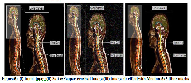Figure 5:  (i) Input Image(ii) Salt &Pepper crashed Image (iii) Image clarified with Median 5×5 filter masks.  Click here to view figure

 

Figure 6:  (i) Input Image (ii) Salt &Pepper crashed Image  (iii) Image clarified with Gaussian 5×5 filter masks. Click here to view figure

 

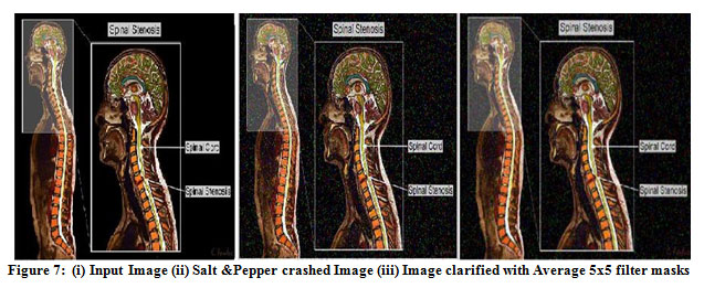Figure 7:  (i) Input Image (ii) Salt &Pepper crashed Image (iii) Image clarified with Average 5×5 filter masks. Click here to view figure

 

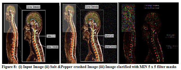Figure 8:  (i) Input Image (ii) Salt &Pepper crashed Image (iii) Image clarified with MIN 5 x 5 filter masks. Click here to view figure

 

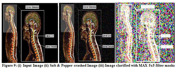Figure 9: (i)  Input Image (ii) Salt & Pepper crashed Image (iii) Image clarified with MAX 5×5 filter masks. Click here to view figure

 

Figure 10:  (i) Input Image (ii) Salt & Pepper crashed Image  (iii) Image clarified with Wiener 5×5 filter masks. Click here to view figure

Restoring Gaussian Noise image using 5 x 5 Windows filters

The figures 11-16 depicts restoration of input image crashed using Gaussian Noise using several 5×5 filter masks to improve clarity of image.

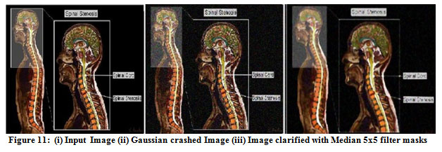Figure 11:  (i) Input Image (ii) Gaussian crashed Image (iii) Image clarified with Median 5×5 filter masks. Click here to view figure

 

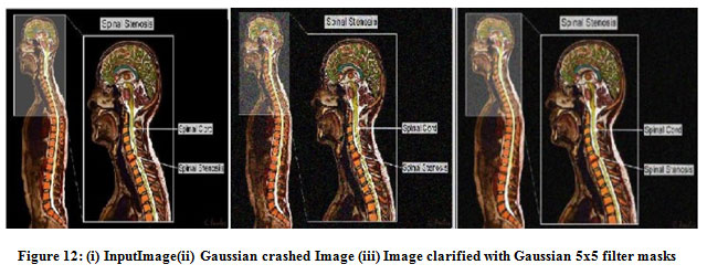Figure 12: (i) Input Image(ii) Gaussian crashed Image (iii) Image clarified with Gaussian 5×5 filter masks. Click here to view figure

 

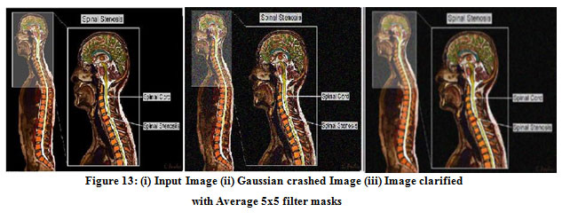Figure 13: (i) Input Image (ii) Gaussian crashed Image (iii) Image clarified with Average 5×5 filter masks. Click here to view figure

 

Figure 14:  (i) Input Image (ii) Gaussian crashed Image (iii) Image clarified with MIN 5×5 filter masks. Click here to view figure

 

Figure 15:  (i) Input Image (ii) Gaussian crashed Image (iii) Image clarified with MAX 5×5 filter masks. Click here to view figure

 

Figure 16: (i) Input Image (ii) Gaussian crashed Image (iii) Image clarified with Wiener 5×5 filter masks. Click here to view figure

Restoring Speckle noise image using 5 x 5 windows Filters

In the figures 17-22 restoration of input image degraded with the addition of speckle Noise using several 5×5 window filters to recover the original image have been presented.

Figure 17:  (i) Input Image (ii) Speckle crashed Image (iii) Image clarified with Median 5×5 filter masks. Click here to view figure

 

Figure 18:  (i) Input Image (ii) Speckle crashed Image (iii) Image clarified with Gaussian 5×5 filter masks. Click here to view figure

 

Figure 19: (i) Input Image (ii) Speckle crashed Image (iii) Image clarified with Average 5×5 filter masks. Click here to view figure

 

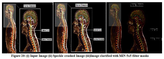Figure 20: (i) Input Image (ii) Speckle crashed Image (iii)Image clarified with MIN 5×5 filter masks. Click here to view figure

 

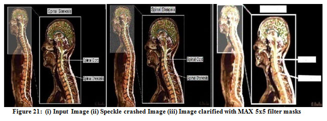Figure 21:  (i) Input Image (ii) Speckle crashed Image (iii) Image clarified with MAX 5×5 filter masks. Click here to view figure

 

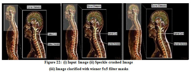Figure 22:  (i) Input Image (ii) Speckle crashed Image  (iii) Image clarified with wiener 5×5 filter masks. Click here to view figure

Restoring poisson Noise image using 5 x 5 Windows Filters

The restoration of image corrupted using poisson noise using various restoration techniques has been achieved  in the figures 23-28.

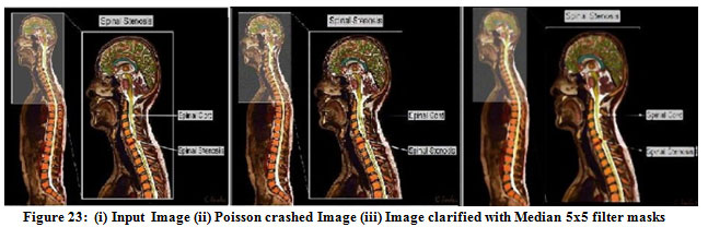Figure 23: (i) Input Image (ii) Poisson crashed Image (iii) Image clarified with Median 5×5 filter masks Click here to view figure

 

Figure 24:  (i) Input Image (ii) Poisson crashed Image (iii) Image clarified with Gaussian 5×5 filter masks. Click here to view figure

 

Figure 25: (i) Input Image (ii) Poisson crashed Image (iii) Image clarified with Average 5×5 filter masks. Click here to view figure

 

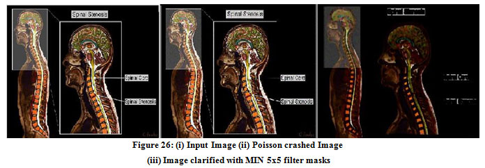Figure 26: (i) Input Image (ii) Poisson crashed Image (iii) Image clarified with MIN 5×5 filter masks Click here to view figure

 

Figure 27: (i) Input Image (ii) Poisson crashed Image (iii) Image clarified with MAX 5×5 filter masks Click here to view figure

 

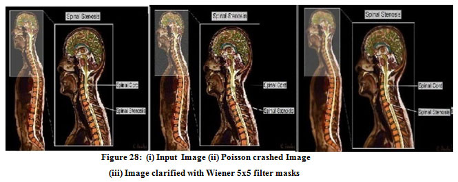Figure 28:  (i) Input Image (ii) Poisson crashed Image (iii) Image clarified with Wiener 5×5 filter masks. Click here to view figure

Filter Performance Analysis

MSE (Mean Square Error)

It has been observed that for salt and pepper noise image of the cervical spine MRI as shown in figures 5-10,the MSE values of Gaussian filter window 5 x 5 is much better than other filters as can been seen in table 1. It can also be observed that wiener filter has provided better performance for degraded 3D cervical spine MRI image using Gaussian,speckle and Poisson noise as presented in table 1.

Table 1: Mean Square Error for 5 x 5 window filters for RGB image

Name of Filter	Type of Noise
	Salt and Pepper	Gaussian	Speckle	Poisson
Median	960.671	931.219	996.432	947.076
Gaussian	561.046	483.578	414.973	358.538
Average	1089.27	1088.03	1032.48	997.02
Min	5626.37	4518.35	4175.24	3929.38
Max	25225.5	7666.69	6060.06	5360.14
Wiener	556.294	303.88	245.605	161.058

PSNR (Peak Signal to Noise Ratio)

In table 2, it has been shown that for corrupted 3D cervical spine MRI images with the addition of salt and pepper, Gaussian, Speckle and Poisson,the wiener filter 5 x 5 window has provided a better peak signal to noise ratio.It can also be analyzed that performance of Gaussian filter with 5 x 5 window is also good or stable for considered corrupted images.

Table 2: Peak Signal to Noise Ratio for 5×5 window filters for RGB image

Name of Filter	Type of Noise
	Salt and Pepper	Gaussian	Speckle	Poisson
Median	18.3051	18.4403	18.1463	18.367
Gaussian	20.6408	21.2861	21.9506	22.5855
Average	17.7595	17.7644	17.992	18.1438
Min	10.6285	11.581	11.924	12.1876
Max	4.1124	9.2847	10.306	10.839
Wiener	20.6778	23.3038	24.2284	26.061

CC (Cross Correlation)

For 3D cervical spine MRI image degraded with Salt and Pepper noise, cross correlation values of Gaussian filter are much better than other filters used to recover the original image as shown in table 3. But cross correlation values of wiener filter 5 x 5 window is much better  than other filters which are used in the proposed work for Gaussian, speckle and Poisson noise image as can be seen in table 3.

Table 3: Cross Correlation for 5 x 5 window filters for RGB image

Name of Filter	Type of Noise
	Salt and Pepper	Gaussian	Speckle	Poisson
Median	0.637	0.61922	0.633	0.637
Gaussian	0.6261	0.61609	0.6592	0.6637
Average	0.5763	0.56211	0.6049	0.6083
Min	0.3715	0.51327	0.5213	0.5164
Max	0.1733	0.37174	0.4931	0.4963
Wiener	0.6309	0.63391	0.6764	0.6828

Conclusion

Image restoration techniques for medical images are not so much developed in the present scenario, but their use for proper application and performance measure is still a matter of ongoing research. In the proposed work, different linear and nonlinear restoration techniques have been applied to noisy images which are corrupted with the addition of Salt and Pepper, Gaussian, Speckle and Poisson noises to recover the image. The quantitative analysis using numerical parameters like MSE, PSNR and CC of linear and nonlinear filters for noisy images has been carried out in this proposed research work.It can be concluded that the Wiener Filter with 5 x 5 window is the best filter for Gaussian, speckle and Poisson noise, according to the experimental results on 3D cervical spine MRI Image. Also, Gaussian filter with 5 x 5 window is the best filter in order to de noise and restores 3D cervical spine MRI image degraded by the addition of salt & pepper noise. The restoration techniques used in the proposed work can be used to retain the structural details of the medical image.

Acknowledgment

None

Funding Source

None

Conflict of Interest:

Authors of the proposed research work  declare that he/she has no conflict of interest.

References

1. James and B.DasarathyMedical image fusion: A survey of the state of the art, Information Fusion, 2014;19: 4-19.
   CrossRef
2. Suhas and C.R. Venugopal, “MRI Image Processing and Noise Removal Technique using Linear and Nonlinear filters”, IEEE International Conference on Electrical, Electronics, Communication, Computer and Optimization Techniques (ICEECCOT) 2017;9:709-712.
   CrossRef
3. R. Banham and A. K. Katsaggelos, Digital image restoration IEEE Signal Processing Magazine, 1997;14: 24–41.
   CrossRef
4. Anmol Sharma and Jagroop Singh Image Denoising using Spatial Domain Filters: A Quantitative Study 6th IEEE International Congress on Image and Signal Processing, 2013;7:293-298 .
   CrossRef
5. Nguyen ThanhBinh and Ashish KhareAdaptive complex wavelet technique formedical image denoising proceedings of the third International Conference on the development of Biomedical Engineering, Vietnam, 2015;195-198.
6. KaurNoise Types and Various Removal Techniques International Journal of Advanced Research in Electronics and Communication Engineering (IJARECE) , 2015; 4:226-230
7. Shinde, D. Mhaske, M.Patare, A.R. DaniApply Different Filtering Techniques To Remove The Speckle Noise Using Medical Images International Journal of Engineering Research and Applications, 2012; 2:1071-1079.
8. Aboshosha, et alImage denoising based on spatial filters, an analytical studyInternational Conference on Computer Engineering & Systems, 2009; .245-250.
   CrossRef
9. CharuKhare and Kapil Kumar NagwanshiImage Restoration Technique with Non-Linear Filter International Journal of Advanced Science and Technology, 2012; 39: 67-44
10. Mahmoud, S. EL Rabaie, T. E. Taha, O. Zahran, F. E. Abd El-SamieComparative study between different denoising filters for speckle noise reduction in ultrasonic B-mode images8th International Computer Engineering Conference (ICENCO), 2012;30-36.
    CrossRef
11. Oge MarquesPractical Image and Video Processing Using MATLAB Wiley, New York, September 21,2011.
    CrossRef
12. M. AliMRI Medical Image De noising by Fundamentals filters High-Resolution Neuro imaging – Basic Physical Principles and Clinical Applications, 2018;111-124.
    CrossRef

(Visited 274 times, 1 visits today)