B.Krishna Kumar

Department of ECE, Methodist College of Engineering and Technology, Hyderabad-500001, Telangana State, India.

Corresponding Author E-mail: saisantu2004@yahoo.co.in

DOI : https://dx.doi.org/10.13005/bpj/2142

Abstract

Electroencephalogram (EEG) is basically a standard method for investigating the brain’s electrical action in diverse psychological and pathological states. Investigation of Electroencephalogram (EEG) signal is a tough task due to the occurrence of different artifacts such as Ocular Artifacts (OA) and Electromyogram. By and large EEG signals falls in the  range of DC to 60 Hz and amplitude of 1-5 µv. Ocular artifacts do have the similar statistical properties of EEG signals, often interfere with EEG signal, thereby making the analysis of EEG signals more complex[1]. In this research paper, Principal Component Analysis is employed in denoising the EEG signals. This paper explains up to what level the scaling of principal components have to be done. This paper explains the number of levels of scaling the principal components to get the high quality EEG signal. The work has been carried out on different data sets and later estimated the SNR.

Keywords

Denoising; Multi Scale PCA (MSPCA); Principal Components; PCA; SNR

Download this article as: 

Copy the following to cite this article: Kumar B. K. Estimation of Number of Levels of Scaling the Principal Components in Denoising EEG Signals. Biomed Pharmacol J 2021;14(1).

Copy the following to cite this URL: Kumar B. K. Estimation of Number of Levels of Scaling the Principal Components in Denoising EEG Signals. Biomed Pharmacol J 2021;14(1). Available from: https://bit.ly/2ZRVCbJ

Introduction

The study of Electroencephalogram is very much helpful in diagnosing different disorders of the nervous system. EEG is the electrical action recorded from the scalp surface, which is picked up by conductive media and electrodes [1-3]. EEG has been performing a vital role in investigating brain activities in clinical application and scientific research for several years [4-6]. The EEG signals can be contaminated by various artifacts, of which the major noise source is ocular artifact, which includes Eye-movement and eye-blink’s [7]. However, artifacts are the major enemies of high-class EEG signals.  The mixing up of these ocular artifacts with the EEG signal at the time of recording causes the problems in the accurate estimation of EEG signal. These artifacts will plunge into either of the 2 categories namely, technical and physiological artifacts. Power line noise 50/60Hz falls into technical artifact category while the artifacts that crop up  because of ocular(EOG), heart(ECG) and muscular activity(EMG)  falls into  physiological artifacts category respectively [8].

Regression in the time domain and frequency domain [9-11] methods were proposed in removing eye blinks artifacts. These methods require a reliable reference channel. This channel can be contaminated by EEG. So, EEG has to be removed from the reference channel by regression techniques. Hence, the regression methods are not the finest to remove EOG artifacts.

Principal Component Analysis is one of the available techniques for extracting the information from the data and has found applications in a wide range of disciplines [12]. PCA  was introduced by Pearson in 1901[13] and developed by Hotelling [14]in the year 1933.

In this research paper, up to how many levels the principal components have to be scaled for obtaining the better denoised EEG signal is elaborated using MSPCA and WAVELETS [15] and later estimated the SNR.

Methodology

Principal Component Analysis

Principal Component Analysis (PCA) can be applied to EEG data that contains a large number of measured variables to develop into a smaller number of artificial variables called principal components(PC). Obtaining a smaller number of variables from a large number of measured variables is to reduce the redundancy in the measured variables. Here, redundancy means some of the variables in the measured data are correlated with one another,because they are measuring the same construct.The main idea of PCA is to reduce the dimensionality of the data set, as the data set consists of a large number of interrelated variables, and trying to retain as much as  possible variation present in the data set.

These principal components are uncorrelated,orthogonal  and ordered in such a way that the first few components retain most variation present in all  of the original variables. PCA is performed by eigen value decomposition of data covariance matrix.This is usually done after mean centering the data for each attribute.

If the variables in a data set are already uncorrelated, PCA is of no value. In addition to being uncorrelated, the principal components are orthogonal and are ordered in terms of the variability they represent. That is, the first principal component represents, for a single dimension (i.e., variable), the greatest amount of variability in the original data set. Each succeeding orthogonal component accounts for as much of the remaining variability as possible.

In other words, Principal component analysis (PCA) is a multivariate data analysis procedure that transforms a set of ‘n’ correlated variables, X = (x₁, x₂… x_n,), into a set of uncorrelated variables called principal components (p₁, p₂, …, p_n). The first principal component accounts for most of the variability in the data, while each of the succeeding components in turn account for the highest amount of the remaining variability. Each principal component is a linear combination of the variables, X. The i^th principal component can thus be expressed as:

y_i = e_i^TX                     ……….        (1)

where,

e_i is the eigenvector of the covariance matrix (R) of X (e_i^T is the transpose of e_i).

The variance of the ith principal component is given by

Var(Y_i) =e_i^T R ;                         (2)

where

e =λ_i;          i = 1, 2. . . n

λ_i  is the i^th   eigenvalue.

PCA makes one stringent but powerful assumption, linearity. This assumption simplifies the problem by restricting the number of variables from the measured data. Hence PCA is used to re-express the data, which is a linear combination of original basis and which is explained here in terms of linear algebra.

Consider an original data set X, which is an mxn matrix, where ‘m’ corresponds to the number of measurement types and ‘n’ is the number of samples. The main goal is to find an orthonormal matrix ‘P’ in Y=PX such that C_Y=1/n(YY^T  ) is a diagonal matrix. The matrix ‘P’ transforms ‘X’ into ‘Y’. The rows of orthonormal matrix ‘P’ represent principal components of original data set ‘X’.

First Level PCA

Two data sets, namely, EEG data set1(X1) and EEG data set2(X2), each of size 1×1000, were collected from physionet.org website [16]. These two data sets were down sampled by a factor of 2. This reduces the size of each data set to 1×500. Each data set is normalized using the following formula:

X=(X-mean(X))/std(X)

where, mean(X) is mean of X

std(X) is standard deviation of X

The mean of each data set is calculated using the following formula:

Where, n corresponds to number of samples in the data set X.

The variance of each data set is calculated using the following formula:

After obtaining the normalized data sets, a noise signal (EOG signal collected from physionet.org website), whose variance is of 0.4 and of length 500, is added to the two data sets. This results in two noisy data sets. These two noisy data sets are of size 1×500 are converted into a column vector.

X=[X1; X2].

The size of the column vector will be equal to 500×2.This column vector is treated as noisy EEG signal. For each column of data matrix wavelet decomposition is done to a level of 6 using sym8 wavelet. The wavelet decomposition gives approximate and detailed coefficients of noisy EEG signal. At each level of wavelet decomposition, i.e., on approximations and as well as details in wavelet domain, corresponding covariance matrices are computed. For each covariance matrix, PCA is performed. After performing the PCA on each covariance matrix, at each level, the most significant Principal Components (PC’S) are selected. Here the selection of Principal Components is done using the Kaiser’s rule. This rule retains the Principal Components that are associated with the Eigen values greater the mean of all Eigen values [17].

The Principal Components at each level of decomposition and corresponding Principal Component variances vectors are provided in the Table 1

Table 1: Principal Components at Each Level of Decomposition and Corresponding Principal Component Variances Vectors-[FIRST SCALE PCA].

Level No	Principal Components Vector At Each Level   (Eigen Vectors)	PC Variances (Eigen Values)
1	-0.71426             0.69987 0.69987              0.71426	0.18818 0.14141
2	0.31328             0.94965 0.94965           – 0.31328	0.23541 0.17906
3	-0.03374          0.99943 -0.99943          -0.03374	0.79591 0.55813
4	0.33820           -0.94107 0.94107           0.33820	4.19395 1.614760
5	-0.46860          0.88341 -0.88341          -0.46860	8.69436 6.47539
6	0.04964           -0.99877 0.99877           0.04964	11.31132 2.59938
7	0.93849           -0.34529 0.34529           0.93849	136.82706 11.83056
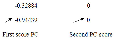
8	-0.32884              0 -0.94439               0	1.12188 0.21859

Principal Components (1.12188 and 0.21859) corresponding to level 8 are the number of retained principal components for final PCA after wavelet reconstruction.

From level 8, it is observed that the original data in two dimensional spaces is reduced to one dimension and shown below for ready reference.

   LEVEL 8

Using these principal components one can reconstruct the denoised version of the input matrix X. The denoised versions of the input matrix X i.e., EEG data set1 and EEG data set2 are shown in the Fig. 1 (a) and Fig. 1(b) respectively.

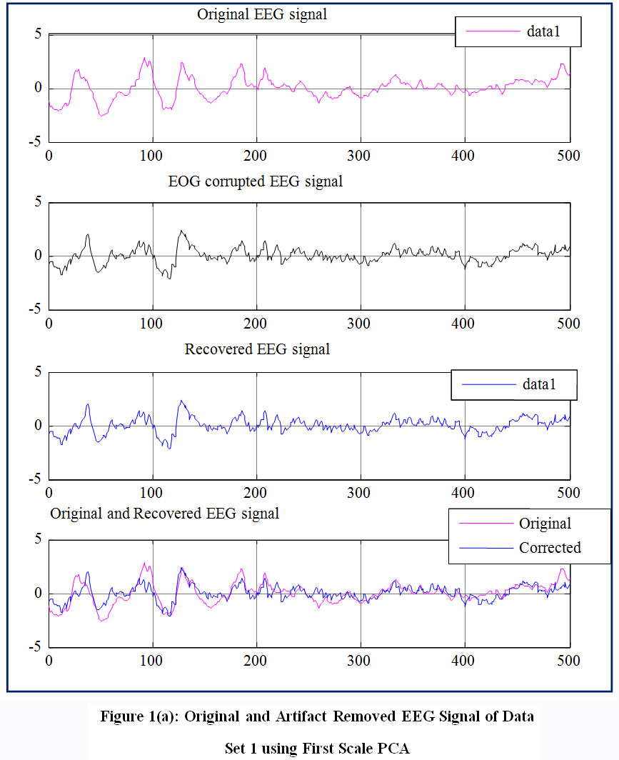Figure 1(a): Original and Artifact Removed EEG Signal of Data Set 1 using First Scale PCA. Click here to view figure

 

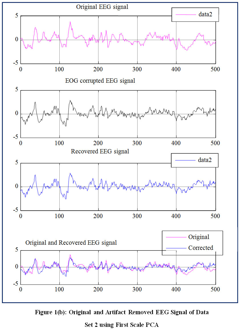Figure 1(b): Original and Artifact Removed EEG Signal of Data Set 2 using First Scale PCA. Click here to view figure

The quality of column reconstructions is estimated by the relative mean square error are 22.1904933458124% and 73.9497428008459%, not closer to 100%.

Since the quality of column reconstructions after first level PCA are not closer to 100%, hence the level of scaling principal components is taken to next level [18]. Hence retaining of principal components will be decided based on the quality of reconstruction of columns which is measured by relative mean square error.

Second Level PCA

The simplified input matrix X, which was obtained from the first scale of PCA, is again decomposed to a level of 6 using sym8 wavelet. Now the wavelet coefficients obtained after the wavelet decomposition are thresholded using Heursure thresholding. For these wavelet coefficients PCA is performed and selected the significant principal components. Using these principal components one can reconstruct the much more denoised input matrix X. The quality of reconstruction of the columns estimated after the second time processing of the input matrix x are close to 100% and are 99.9981% and 99.9991%.

The principal components and Principal Component variances vectors of the two data sets obtained after second scale PCA and wavelet denoising are shown in the Table.2.

Table 2: Principal Components and Principal Component Variances Vectors Obtained After Second Scale PCA and Wavelet Denoising.

Level No	Principal Components Vector At Each Level (Eigen Vector)	PC Variances (Eigen value)
1	-0.74792          -0.66378 -0.66378          0.74792	0.17755 0.14424
2	-0.47075          -0.88226 0.88226             -0.47075	0.18846 0.17321
3	-0.03589          -0.99936 0.99936           -0.03589	0.73933 0.43569
4	0.45131             0.89237 0.89237           -0.45131	4.01686 1.39216
5	0.78691               0.61707 0.61707              -0.78691	9.15681 5.49690
6	0.04293              -0.99907 0.99907              0.04293	11.28581 2.15695
7	0.93978               0.34178 0.34178           -0.93978	175.29829 6.19914
8	0.58069                            0 0.81412                            0	1.27604 0.28103

Principal Components (1.27604 and 0.28103) corresponding to level 8 are the number of retained principal components for final PCA after wavelet reconstruction.

From level 8, it is observed that the original data in two dimensional spaces is reduced to one dimension and shown below for ready reference.

Level 8

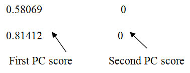
On comparing Table.1 and Table2  the final PC’s in the level 8 are improved after second time PCA using wavelet denoising [19].Using the selected principal components one can reconstruct noise free EEG signals back. The waveforms of Denoised EEG signal constructed after second scale PCA are shown in Fig 2(a) and 2(b).

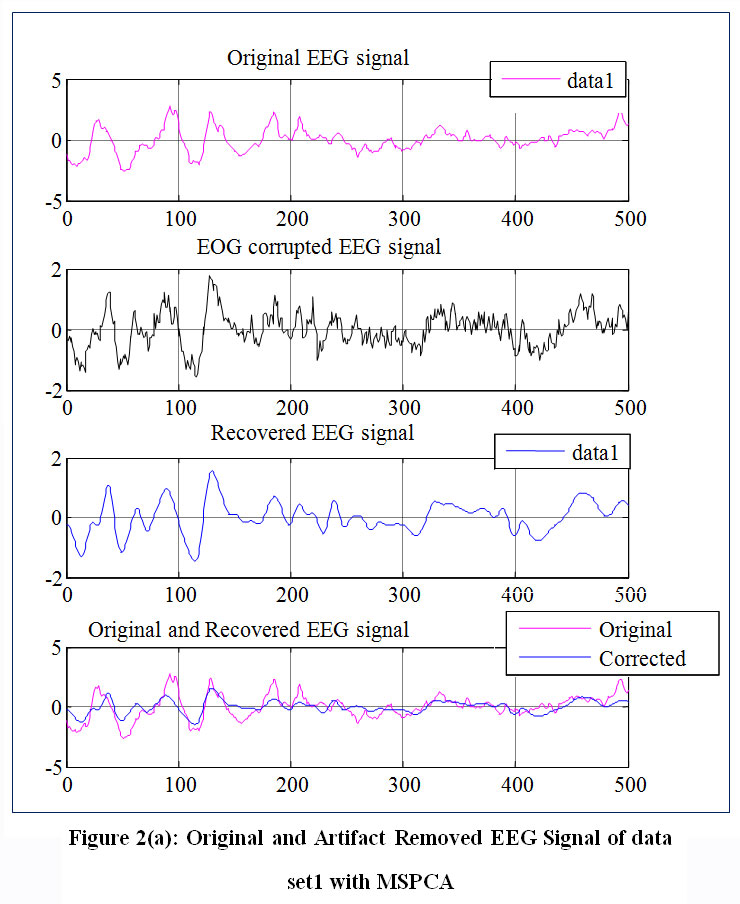Figure 2(a): Original and Artifact Removed EEG Signal of data set 1 with MSPCA Click here to view figure

 

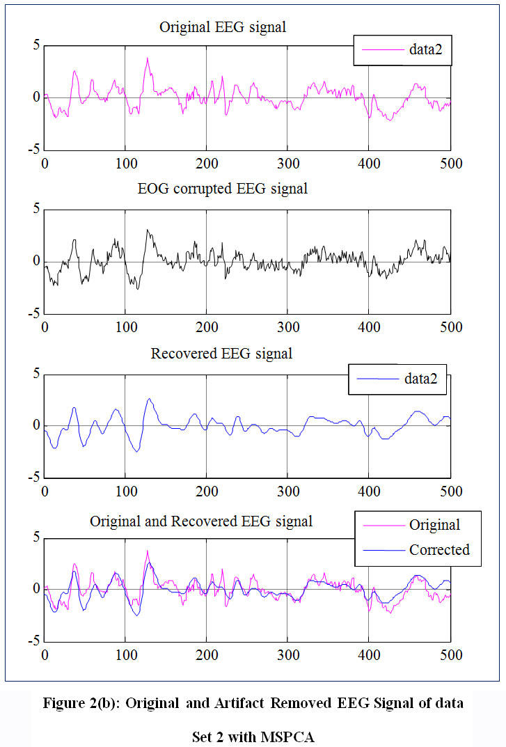Figure 2(b): Original and Artifact Removed EEG Signal of data Set 2 with MSPCA. Click here to view figure

Results

The results obtained after performing MSPCA on different data sets were tabulated in Table 3 and also compared with the previous results [18].

Table 3: Comparison of SNR of Denoised EEG Signal Obtained using MSPCA and Different Wavelets.

	Wavelet family/Threshold type	SNR (dB)
1)B Krishna Kumar Analysis of EEG Signals Using Multi-Scale Principal Component Analysis- 2) B. K. Kumar and K. V. S. V. R. Prasad, “Performance comparison of IST and multi scale principal component analysis in the EEG signal processing,” 2017 International Conference on Computing Methodologies and Communication (ICCMC)	Sym8 (soft)	34.95
	Sym8 (hard)	24.52
	Haar (soft)	20.29
	Haar (hard)	25.10
	dB10 (soft)	28.89
	dB10 (hard)	23.74
Proposed method	MSPCA ( for DATA SETS-1 AND 2)	37.43
Proposed method	MSPCA( for DATA SETS-2 AND 3)	35.36
Proposed method	MSPCA( for DATA SETS -4 AND 5 )	35.16

Conclusion

The MSPCA is providing better SNR as the Relative Mean Square Error(RMSE) of the columns is closure to 100%. Hence, it is important to check the Relative Mean Square Error (RMSE) of the columns before reconstructing the Denoised EEG signal and estimating the SNR.

Acknowledgement  

Not applicable

Conflict of Interest                            

There is no conflict of interest.

Funding Source                                 

Not applicable

References

1. Krishna Kumar “ Denoising of EEG Signals using Wavelets and SIMULINK Techniques “International Journal of Recent Technology and Engineering (IJRTE) , Volume-8 Issue-5, January 2020 pp.335-339
   CrossRef
2. E.Niedermeyer and FH Silva. “Electroencephalography: Basic principles, clinical applications and related fields”, Lippincott, Williams & Wilkins, (2004),
3. MR Arab, AA Suratgar, VMM Hernandez, AR Ashtiani “Electroencephalogram Signals Processing for the Diagnosis of Petit mal and Grand mal Epilepsies Using an Artficial Neural Network.Journal of Applied Research and Technology, 8 (2010), pp. 120-129.
   CrossRef
4. GL Holmes, ad CT Lombroso. “Prognostic value of background patterns in the neonatal EEG”.J. Clin. Neurophysiol, 10 (1993), pp. 323-352
   CrossRef
5. S Almubarak, and PK Wong.” Long-Term Clinical Outcome of Neonatal EEG Findings’           J.Clin.Neurophysiol,28(2011),pp.185- 189http://dx.doi.org/10.1097/WNP.0b013e3182121731 | Medline
   CrossRef
6. ASM Muthanantha Murugavel, S Ramakrishnan.”Tree Based Wavelet Transform and DAG SVM for Seizure Detection.Signal and Image Processing”: An International Journal, 3 (2012), pp. 115-125
   CrossRef
7. N.V. Thakor et al. (1993). “Multi resolution Wavelet Analysis of Evoked Potentials”, IEEE Transactions on Biomedical Engineering, Vol. 40, No 11, pp. 1085-1093,November.
   CrossRef
8. S. Ventakaramanan, P. Prabhat, S.R Choudhury, H.B Nemade, and J.S. Sahambi. (2000). “Biomedical Instrumentation Based On Electrooculogram (EOG) Signal Processing And Application To A Hospital Alarm System”, Indian Institute Of Technology (IIT) Gauhati, Proceedings of IEEE ICISEP, pp.535-539.
9. Schlogl A, Keinrath C, Zimmermann D et al. 2007. A fully automated correction method of EOG artifacts in EEG recordings. Clinical Neurophysiology.118, 98–104.
   CrossRef
10. Jung T-P, Makeig S, Humphries C, Lee T-W, McKeown MJ,Iragui V and Sejnowski TJ. 2000a. Removing Electroencephalographic artifacts by blind source separation.Psychophysiology.37, 163 –178.
    CrossRef
11. Gratton G, Coles MG and Donchin E. 1983. A new method for off-line removal of oucular artifact. Electroencephalography Clin.Neurophysiol. 55, 484– 486.
    CrossRef
12. M.Aminghafari,N. cheze, J.M Poggi, ”Multivariate denoising using wavelets and principal component Analysis,” computational statistics & Data Analysis, vol. 50 pp. 2381-2398,2006.
    CrossRef
13. Pearson, K, “On Lines and Planes of Closest Fit to Systems of Points in Space”, Phil. Magazine, vol.6, issue. 2, pp.559–572, 1901.
    CrossRef
14. Hotelling. H,” Analysis of a Complex of Statistical Variables Into Principal Components”, J. Educ. Psychol., 24, pp.417–441, pp.498–520, 1933.
    CrossRef
15. B. K. Kumar and K. V. S. V. R. Prasad, “Performance comparison of IST and multi scale principal component analysis in the EEG signal processing,” 2017 International Conference on Computing Methodologies and Communication (ICCMC), Erode, 2017, pp. 536-542, doi: 10.1109/ICCMC.2017.8282523.
    CrossRef
16. www.physionet.org
17. www.mathworks.com/products/matlab/, Discrete Wavelet Transform-2010.
18. B.KrishnaKumar ,Dr.K.V.S.V.R.Prasad, Dr.K.Kishan Rao  and  Narsimha Baddiri, “Analysis of EEG Signals Using Multi-Scale Principal Component Analysis”, IEEE Conference, Cape Institute of Technology, Levingapuram, Kanyakumari, pp.359-363, December15-18, 2011.
19. W.M.Bukhari W, Daud and Rubita Sudirman, “Time Frequency Analysis of Electrooculography (EOG) Signal of Eye Movement Potentials Based on Wavelet Energy Distribution”,2011 Fifth Asia Modeling Symposium, pp.81-86,2011.

(Visited 294 times, 1 visits today)