Anaahat Dhindsa^1,3, Sanjay Bhatia², Sunil Agrawal³ and B.S. Sohi⁴

¹Department of Electronics and Communication Engineering, Chandigarh University, Gharuan, Punjab, India,140413, 0000-0003-3877-6851

²Department of Zoology, University of Jammu, India, 180016

³UIET, Panjab University, Chandigarh, India, 160014

⁴Chandigarh University, Gharuan, Punjab, India, 140413

Corresponding Author E-mail : anaahat.dhindsa85@gmail.com

DOI : https://dx.doi.org/10.13005/bpj/1979

Abstract

This research work is motivated by a need to focus on computational biodiversity studies, to contribute towards research in maintaining the ecological balance of the earth. The field of computational biodiversity can leverage current advents in image processing and machine learning algorithms. This paper gives information on how to develop a pipeline of algorithms that can support biodiversity studies. The process of manual identification of algae in water bodies is tedious and laborious, and highly dependent on experts. The work demonstrated here provides methods to resolve this problem by automating the process. A hybrid algorithm that uses pixel clustering and Kirsch filter for extracting the bodies of microbes from images has been developed with high accuracy. For the automatic identification process, extensive study is done on comparing Classification and Regression Trees (CART), K-nearest- neighborhood, Gaussian Naive Bayes, Linear Regression, Linear discriminant analysis and Support vector classifier (SVC) methods. This study shows that CART algorithm is the most stable and consistent performer which is evident from the values of recall, precision, and accuracy. The SVC algorithm was second in performance.

Keywords

Algae; Classifiers; Computational Biodiversity; Image Segmentation

Download this article as: 

Copy the following to cite this article: Dhindsa A, Bhatia S, Agrawal S, Sohi B.S. An Efficient Microbes Detection System using Microscopic Images via Morphological and Correlation Based Features. Biomed Pharmacol J 2020;13(3).

Copy the following to cite this URL: Dhindsa A, Bhatia S, Agrawal S, Sohi B.S. An Efficient Microbes Detection System using Microscopic Images via Morphological and Correlation Based Features. Biomed Pharmacol J 2020;13(3). Available from: https://bit.ly/31iVtzD

Introduction

There has been a rapid development of methods aimed at detecting microorganisms.¹ It is a well-established fact that these microorganisms are indicators of human health.² Algae communities exemplify many indicators of ecological balance.³ The study of their diversity can give hints about the water quality, nutritional level of the water body and concentration of pollutants. Algae are ideally suited for health assessment because the chemical and physical properties of the water bodies may help in understanding the levels of pollution in the water, but would fail to give an assessment of the anthropogenic stress under which the biodiversity is going through. There are many studies focusing on the harmful algal blooms that happen due to human activities and due to changes in ecological balances.⁴ Due to these concerns, the golden standard to study such problems is to start with the identification of microorganisms that are causing ecological imbalance.⁵ The identification typically begins with enumeration of microorganisms under microscope, and identification using an expert in the field. Many scholars^{6 7} have developed methods and procedures on how to measure the quality of water based on the types of microorganisms it contains, especially in the context of drinking water for classifying the percentage of microorganisms that are contained in the water.

The domain of computational biodiversity comes under the purview of computational biology or bioinformatics.⁸ The main challenge here is the difficulty felt by the researchers in defining the expanse of the study area. The biodiversity studies can be done on any scale.⁹ It can be done in an area as small as a compost pit, and as big as a tropical rainforest. The shape, color and habitat differences make the process of computing biodiversity interesting but challenging, and need the expert help of taxonomists.¹⁰ It is even harder to automate the process initially because each species may require a different computational algorithm for segmenting it from the microscopic slides.¹¹ If the segmentation of the region of interest (ROI) is not accurate enough, then the machine learning algorithms will be fed with noisy data leading to less robust automation.¹² If similar shape features are going to be used, there is a high possibility that the characteristics will have a high degree of correlation.¹³,¹⁴ This can lead to unnecessary information overload. Moreover, another issue is collection, segregation, grading and segmentation of images. During segmentation, removing noise and artifacts is a big challenge. This process can be improved by employing methods that can create clean and clear slides.¹⁵

The outcome of a biodiversity study is greatly impacted by the quality of sampling and measurements taken by the sample collector.³ If the collection of the samples is not done as per the protocols and guidelines, the outcome of the process may lead to incorrect statistical results. The collected data of microorganisms may not be “balanced”.¹⁶ In simple words, the dataset may not have an equal proportion of information of all the species under study.

In this research work, the focus is to reduce the workload of taxonomists by automating the process of identification of algae. The focus of the study will be two water bodies located in Chandigarh, an urban area, where deterioration of their health is a concern for scientific communities.^17,18 This study investigates the feasibility of the different image segmentation methods and machine learning models to automate the process of identification of algae. Hence, we intend to resolve the two main problems that previous algorithms have been facing in the context of building an automated system of identification. The first problem is about the issue of collinearity and the second issue is the problem of having an unequal proposition of class wise data points i.e. unbalanced dataset.¹⁶ Hence, to solve these two main issues this work has been undertaken to construct a generic segmentation algorithm for segmenting bodies of at least ten algae species by using its shape characteristics. Many previous algorithms have been using color, texture or features that are based on characteristics of pixels of the images and a limited attempt has been made to map the shapes of the algae with machine learning features. In addition, there is limited work done to handle the problem of unbalanced datasets that can lead to bias and sub-optimal outcomes of the machine learning algorithms. Hence, in the proposed work an attempt is made to handle the imbalanced dataset automatically so that the overhead remains low. Many authors give evidence that logistic Regression (LR) and Decision Tree (DT) based classifiers undergo a problem of collinearity,^19,20,21 which leads to over fitting. There is a need to make algorithms learn faster, and to reduce the high degree of bias in performances. Hence, the need for hyper-parameter fine-tuning and optimization of the classifiers is essential in the current context. This is primarily done with the help of feature engineering and using cross-validation methods.^22,23,24 Fine-tuning of machine learning algorithms is proposed in order to automatically remove the variables that have similar coefficients due to high correlation in order to remove the duplication of information and unnecessary load on the machine learning algorithms.²⁵ The work however, will be limited to the identification of algae species. The process starts with the collection of water samples from the water bodies, followed by development of whole mounted (WM) slides. The next steps include evaluation, optimization, pipelining of image processing with machine learning algorithms for constructing algorithms of algae identification and classification. The outcome will be a fine-tuned framework of algorithms that will be able to solve the problem of the unbalanced datasets and collinearity automatically.

The paper is organized in multiple sections. Section 2 and 3 gives information on materials and methodology used in this research work. Section 3 has three sub parts. The first subpart discusses the image processing operations, the second subpart discusses about how the segmented images are subjected to feature extraction, and the description of the features dataset is also given. The third subpart gives information on Correlation based feature analysis. Section 4 gives outcomes and results of the work done till now. The results section is followed with the discussion on it. After the discussion, validation of the outcomes is given. A comparative view of the current work with other author’s work is given in section 7. The paper concludes all about its findings in the section 8.

Material

This section gives information on the collection of water samples, preparation of microscopic slides and finally generating the data set that will be used for training machine learning algorithms.

Sample Collection and Data Set Characteristics (Primary Collection)

The water sampling has been done at the littoral zones of Sukhna and Dhanas lakes, India i.e. collection from the surface water near the banks. Both of these lakes have small ephemeral ponds around their periphery and certain parts of the lake can be termed as bogs. Sampling from these areas was also done. Sukhna Lake is a water reservoir of Shivalik foothills, fed by rain along with seasonal streams. A catchment area is developed to avoid direct silting of the Sukhna Lake. Therefore, an area close to 25 square kilometers is covered with vegetation to act as a catchment area. Dhanas Lake is another man-made water body and is smaller in size as compared to Sukhna Lake. Visually, it can be observed that Dhanas Lake has a higher concentration of nutrition or pollutants as compared to Sukhna. This can be attributed to the greenish color of the water. For our study, about ten water sample collection points have been identified for each lake. The dataset consists of images for 10 different algae species, identified with help of reference manuals and experts. The slide preparation was done using a technique in which organic solvents (xylene and benzyl alcohol/benzyl benzoate (BABB)) were used as a diluting agent, which improved light penetration and transparency of the microorganisms while preparing a fully mounted slide. The slides were captured using a microscope at magnification levels of 4x and 10x. Three thousand slides were made, but out of those 620 images qualified as useful images. The reason for using the completely mounted images is that the images will have the least amount of noise for our research work.

Methodology

This section gives information on all the steps taken to overcome the challenge of doing manual identification with help of image processing and machine learning. For better understanding of the flow of research work, Figure 1 can be referred.

Image Processing and Segmentation

The image processing consists of two steps. In this first step the gray scale images of the microbes are subjected to the pixel clustering. This removes unwanted pixels from the image. In this second step, boundaries of the microbes are extracted.

For segmenting microbes from the images, Global Thresholding methods ²⁶ are applied to collect and group the pixels that have intensity greater than threshold, found by automatic thresholding methods. Two types of methods were compared viz, Isodata²⁷ and Otsu.²⁸ In the Otsu method, the process of pixel clustering reduces the combined spread (intra-class) and increases the inter-class spread. An exhaustive searching method identifies a threshold automatically to minimize the weighted sum of variances of the two classes. In the Isodata method, the algorithm first assigns an arbitrary initial cluster vector and then starts collecting similar pixels. This continues until a change in intensity occurs. It continues to do pixel clustering based on merging groups using target threshold value and splitting based on the change in standard deviation. It was found that the Otsu method works well in the context of our problem. It helps to repair and recover some of the pixels that were lost due to the application of filters and makes the boundaries structurally aligned. This is evident from the accuracy metric (Intersection over union ²⁹) values computed to evaluate these algorithms as shown in Table 1.

Table 1: Accuracy of Clustering Algorithms

Algorithm	Random Sample Size			Average IoU Accuracy
	20	40	60
Otsu	17/20 =0.85	38/40 = 0.95	55/60 =0.92	0.91
Isodata	15/20 = 0.75	33/40 = 0.82	50/60 = 0.83	0.80

 

It can be observed that in each evaluation run of different sample sizes, Otsu method scores higher in terms of accuracy. The segmentation output can be observed from Table 2. To maintain brevity of the research work, partial results are shown. The table shows the output of two steps executed in each class of algae. The Otsu method automatically computed the threshold for each microbe that resulted in highly accurate segmentation of the boundaries of the microbes. In the next step, Kirsch Filter ³⁰ is applied to the output images obtained from Otsu method in order to extract the boundaries of the microbes. The role of preprocessing steps such as contrast enhancement also helped to achieve excellent quality of segmented images. The images are then subjected to morphological /shape feature extraction process to build the automated process of identification. The next section discusses this aspect.

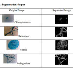Table 2: Segmentation Output Click here to View Table

 

Classifiers for Automation

In this section, the explanation regarding the automatic classification of algae is given. The section begins with the features that will be used for the identification and classification of different algae. There are ten algae species involved in this research work,viz., Chlamydomonas, Cladophora, Nostoc, Oedogonium, Oscillatoria, Pithophora, Spirogyra, Ulothrix, Vaucheria, and Volvox. The data characteristics of the algae dataset shows that Volvox has a maximum proportion of data instances as compared to others. In simple words, it is a clear case of an unbalanced dataset.

The next section gives information on how the features were selected with the help of correlation. For a better understanding of the process, Figure 1 can be referred, which shows the steps to evaluate and validate the different machine learning models. It is also noteworthy here that the choice of the machine learning algorithms for the said purpose is based on the nature of the feature dataset and the problems it embodies. The preliminary examination of the feature dataset shows that the dataset suffers from a high level of collinearity, although each feature is non-linear in nature.

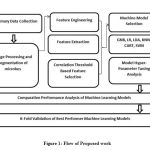Figure 1: Flow of Proposed work Click here to View Figure

 

Feature Dataset Characteristics

In the context of the problem undertaken here, the image(s) is considered as a matrix from which features or the characteristics of the microorganisms are extracted and subjected to machine learning algorithms. From the descriptive statistics of the feature dataset, it was clear that microorganism Volvox has the highest number of feature rows and microorganism Chlamydomonas has the lowest number of feature rows. Hence, it is an unbalanced dataset. To overcome this issue, either resampling needs to be done to balance the number of instances, or there is a need to select a machine-learning algorithm that can take care of the unbalanced dataset. For this reason, we shall proceed to do evaluation of multiple types of algorithms so that we find an appropriate algorithm by doing hyper-tuning of the algorithms. The next step, however, is feature extraction from the images. For this, twenty-five features that describe the shape of microbes were selected. Features such as area (filled and convex) , bounding box ,perimeter, and centroid can give an idea about the shape , size of the microorganism as well as the position of the object in the vector space model.³¹ Features such as equidistant and radii length can provide information between the various parts of the algae. The values of minor and major axes and orientation (tan angle) gives information about the direction and inclination in which the object geometrically is ³². Features such as Convex Hull gives triangulated information about the shape, size, and volume of the algae. The eccentricity feature can help to measure the roundness of the algae object, which again gives indication about the morphology of objects ³³. The feature Extrema is defined as a point, where the value of a number is the largest or smallest in computational space. The feature Extend is computed as the ratio of the pixel area of a region with respect to the bounding box area of an object. Solidity is calculated by dividing the feature area with the convex area.³⁴ The feature Euler number is a value that can be obtained after the subtraction of a number of holes in an image from the total objects in an image.

Feature Correlation Analysis

Theoretically, adding more features should help in improving the ‘discriminate power’ of the dataset. But this is not always true, especially when the features have some degree of associative relationships among themselves. There is a need to eliminate features that add overhead rather than adding discriminate power. Correlation is one of the reliable methods to eliminate irrelevant features, especially when the correlation among the attributes is complex and high in nature. Correlation and covariance are the two main ways based on which the selection of the features is done. Methods such as t-test, p-test, and chi-square methods would yield similar results as correlation.³⁵ Hence, correlation was chosen as criteria for selecting features. The correlation can be computed using Pearson correlation formula as shown in Equation (1).

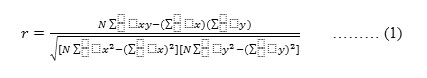
where

N   = number of pairs of scores.

∑xy = sum of the products of paired scores.

∑x  = sum of x scores.

∑y  = sum of y scores.

∑x2  = sum of squared of x scores.

∑y2  = sum of squared of y scores.

The machine learning algorithms were subjected with different sets of features. The sets of features were made with respect to three threshold values (0.85, 0.90, and 0.90). From Table 3, it can be observed that as the correlation threshold value decreases, the number of features to be dropped increases. At the threshold value of 0.95, the number of features dropped is seven for the construction of machine learning since they have a high degree of collinearity. At the threshold value of 0.90, two additional features (‘Major_ Axis_ Length’, ‘Area’)  need to be eliminated from the last set of selected features. Finally, at the correlation threshold 0.85, the number of features that are finally selected are 13. Equipped with these facts, six classification algorithms were further investigated for their performance.

Table 3: Features as per Correlation Threshold

Correlation	Threshold	Features
High Correlation	0.95	‘BoundingBox1’, ‘ConvexHull1’, ‘ConvexHull2’, ‘ConvexHull3’, ‘ConvexHull4’, ‘Centroid1’, ‘Centroid2’
	0.90	‘BoundingBox1’, ‘ConvexHull1’, ‘ConvexHull2’, ‘ConvexHull3’, ‘ConvexHull4’, ‘MajorAxisLength’, ‘Centroid1’, ‘Centroid2’, ‘Area’
Medium Positive  Correlation	0.85	‘Extent’, ‘BoundingBox1’, ‘ConvexHull1’, ‘ConvexHull2’, ‘ConvexHull3’, ‘ConvexHull4’, ‘MajorAxisLength’, ‘Perimeter’, ‘ConvexArea’, ‘Centroid1’, ‘Centroid2’, ‘Area’
Low Positive Correlation	Less than 0.85 and greater than 0.5	‘Solidity’, ‘Eccentricity’, ‘EquivDiameter’, ‘Extrema’, ‘FilledArea’,‘Orientation’, ‘EulerNumber’, ‘BoundingBox2’, ‘BoundingBox3’, ‘BoundingBox4’, ‘MinorAxisLength’, ‘raddi’
Very Low Correlation	Less than 0.5 to 0	‘Solidity’, ‘Eccentricity’, ‘EquivDiameter’, ‘Extrema’, ‘Orientation’, ‘BoundingBox2’ ‘microorganism code’
Negative /Neutral Correlation	Less than 0.001	Solidity

 

The selection of six algorithms is based on the facts collected from literature survey and secondly, it is based on the logic that there is a need to evaluate at least one type of algorithm from different categories of algorithms [Table 4].

Table 4: Machine Model Selection Criteria

S.No	Classifier Category [54][55][56]	Algorithm
1	Probability-based	Gaussian Naïve Bayes (GNB)
2	Distance-Based	K-Nearest Neighbor (KNN)
3	Tree-Based	Decision Tree (CART)
4	Kernel Trick Based	Support Vector Classifier/Machine (SVC/M)
5	Regression Based	Logistic Regression (LR), Linear Discriminant Analysis (LDA)

 

The best performer will be the classifier that handles unbalanced dataset and collinearity with consistently accurate results over multiple validations runs.

Results  

The objective was to find an optimized algorithm that can be used for classification of ten algae species with minimum number of features and overhead. All the algorithms were given features set at 0.85, 90 and 0.95. When the correlation threshold was 0.85, 12 features were dropped and evaluation demonstrated that the CART algorithm has maximum accuracy of 0.98 and SVC had an accuracy of 0.85. Also, a difference of 1 percent can be seen in favor of CART when recall and F1- score values are checked. Algorithms such as GNB, LR, and LDA perform poorly in terms of all evaluation parameters. The recall value of the CART is 0.98 and KNN is 0.90, hence it lags by 0.08 points. The F-score of CART is 0.99 which is close to the ideal value of 1. F-score is a weighted average of recall and precision metrics, hence it clearly shows that both SVC and CART are able to find a good trade-off between recall and precision values. This may be attributed to the fact that in the case of SVC, all the data is transformed into a linear form. At the correlation threshold value of 0.90, only 16 variables were required to be accounted for in machine learning modeling. The outcomes of this series shows that CART has the highest value of F1 score and SVC has a value close to 0.98. Based on this fact, it can be inferred that the CART classifier is stable in terms of recall and precision. At this level of correlation threshold, by adding three more shape features, the accuracy level of the SVC (0.90) increases, whereas in case of CART it remains stable (0.98). It is clear that the performance of CART is repeatable with even less number of features. It was also found that the GNB algorithm could not fit well in the context of classifying ten algae species. At correlation value of 0.95, two more features were added to the last set of selected features in order to check any difference in the performance of all models. Now, we had a maximum number of features (18) to improve the discriminant power of the dataset. At this level also CART was found to be the best performer.

From the tabulated results shown in Table 5 and Table 6, it can be inferred that there is no need to have more than 13 features. This is because adding more than 13 features does not yield any additional benefits. Hence it is concluded that the best features for high level of accuracy with lowest false alarm are ‘Solidity’, ‘Eccentricity’, ‘EquivDiameter’, ‘Extrema’, ‘FilledArea’, ‘Orientation’, ‘EulerNumber’, ‘BoundingBox2’, ‘BoundingBox3’, ‘BoundingBox4’, ‘MinorAxisLength’, ‘raddi’, ‘microorganism code’.

Table 5: Evaluation of GNB, KNN and LDA at different levels of correlation threshold

Algorithm	Model Number	Threshold	Features Selected	Accuracy	Recall	Precision	F1-score
GNB	1	0.30	5	0.25	0.12	0.25	0.16
GNB	2	0.40	6	0.29	0.26	0.3	0.25
GNB	3	0.45	6	0.29	0.26	0.3	0.25
GNB	4	0.50	7	0.36	0.35	0.37	0.34
GNB	5	0.60	8	0.37	0.37	0.37	0.35
GNB	6	0.70	8	0.35	0.37	0.37	0.35
GNB	7	0.80	12	0.19	0.33	0.19	0.15
GNB	8	0.85	13	0.22	0.22	0.33	0.17
GNB	9	0.90	16	0.16	0.16	0.38	0.12
GNB	10	0.95	18	0.14	0.14	0.34	0.1
LDA	11	0.30	5	0.24	0.12	0.25	0.16
LDA	12	0.40	6	0.38	0.37	0.38	0.35
LDA	13	0.45	6	0.34	0.32	0.35	0.31
LDA	14	0.50	7	0.35	0.31	0.35	0.31
LDA	15	0.60	8	0.34	0.32	0.35	0.31
LDA	16	0.70	8	0.34	0.32	0.35	0.31
LDA	17	0.80	12	0.38	0.37	0.38	0.35
LDA	18	0.85	13	0.40	0.4	0.4	0.37
LDA	19	0.90	16	0.40	0.4	0.38	0.38
LDA	20	0.95	18	0.41	0.41	0.4	0.39
KNN	21	0.30	5	0.91	0.91	0.91	0.9
KNN	22	0.40	6	0.91	0.91	0.91	0.9
KNN	23	0.45	6	0.90	0.91	0.91	0.901
KNN	24	0.50	7	0.90	0.91	0.91	0.901
KNN	25	0.60	8	0.91	0.91	0.91	0.9
KNN	26	0.70	8	0.91	0.91	0.91	0.91
KNN	27	0.80	12	0.89	0.9	0.901	0.901
KNN	28	0.85	13	0.90	0.9	0.9	0.90
KNN	29	0.90	16	0.91	0.91	0.91	0.91
KNN	30	0.95	18	0.91	0.91	0.91	0.91
LR	31	0.30	5	0.24	0.12	0.25	0.15
LR	32	0.40	6	0.29	0.22	0.3	0.23
LR	33	0.45	6	0.29	0.22	0.3	0.23
LR	34	0.50	7	0.36	0.33	0.36	0.31
LR	35	0.60	8	0.36	0.33	0.36	0.31
LR	36	0.70	8	0.35	0.3	0.35	0.3
LR	37	0.80	12	0.36	0.3	0.35	0.35
LR	38	0.85	13	0.37	0.37	0.34	0.32
LR	39	0.90	16	0.38	0.38	0.36	0.34
LR	40	0.95	18	0.39	0.39	0.38	0.35

 

Table 6: Comparative Analysis (SVC & CART)

Algorithm	Model  Number	Threshold	Features Selected	Accuracy	Recall	Precision	F1-score
SVC	41	0.30	5	0.84	0.79	0.90	0.86
SVC	42	0.40	6	0.84	0.79	0.90	0.86
SVC	43	0.45	6	0.84	0.79	0.90	0.86
SVC	44	0.50	7	0.842	0.81	0.91	0.86
SVC	45	0.60	8	0.8425	0.80	0.92	0.86
SVC	46	0.70	8	0.8428	0.85	0.94	0.89
SVC	47	0.80	12	0.8428	0.88	0.86	0.87
SVC	48	0.85	13	0.85	0.97	0.98	0.98
SVC	49	0.90	16	0.901	0.97	0.98	0.98
SVC	50	0.95	18	0.95	0.97	0.98	0.98
CART	51	0.30	5	0.9321	0.95	0.84	0.91
CART	52	0.40	6	0.9333	0.90	0.92	0.91
CART	53	0.45	6	0.96	0.98	0.98	0.98
CART	54	0.50	7	0.96	0.98	0.98	0.98
CART	55	0.60	8	0.97	0.98	0.98	0.98
CART	56	0.70	8	0.97	0.98	0.98	0.98
CART	57	0.80	12	0.97	0.98	0.98	0.98
CART	58	0.85	13	0.98	0.98	0.98	0.99
CART	59	0.90	16	0.98	0.98	0.98	0.99
CART	60	0.95	18	0.98	0.98	0.98	0.99

 

Hyper-parameter tuning of SVC and CART was done to arrive at the most optimal parameters that gives maximum level of performance. In case of SVC, the most optimal values for gamma and c were found out to be 2.8 and 1 respectively. The above table gives information on SVC radial optimized with these values. In case of CART, the depth value of 5 gave the best performance.

Discussions

It can be seen that CART seems to be the best-suited algorithm for solving the problem of classification of 10 algae, followed by SVC since its f – score is slightly less than CART. However, it must be noted that CART has more advantages as compared to SVC in terms of selecting features, handling unbalanced data and scaling up on the volume of data. To further investigate this fact, the value of all the performance metrics was also checked at the correlation threshold 0.30 to 0.80. It was found that the accuracy of the SVC algorithm drops about 10% to 13 % approximately. Hence, it is clear that at a threshold value of 0.85, CART gives maximum possible accuracy (0.98) and stable performance. Therefore, to arrive at a decision on the final selection of the best algorithm for the said problem, there is a need to do objective validation. The next section gives information on the application of the 10 -Fold validation process to finally arrive at the selection of the best machine-learning model for algae classification problem.

Validation

The purpose of the K-Fold validation is to estimate the skill of the machine-learning model based on the new dataset; a dataset other than the training dataset. By taking a sample of instances as a holdout or as a test data set and rest (k-1 group(s)) as the training dataset. After the split, the algorithms are run to fit the model in question with these new sets. The values are retained for computing the average score with ‘n’ number of rounds. In context of our research work K= 10, which implies that the validation/testing ratio is 10% and training ratio will be 90%. The box-plot in Figure 2 was plotted and values displayed were calculated using the Interquartile Range (IQR) method. From the shape of the box-plot of the CART, it can be inferred that it has the tightest range, hence, it is more stable in performance. It can be safely inferred that the CART is giving a numerically stable performance at a correlation threshold of 0.85 with minimum features. The process can be designated as repeatable and reproducible.

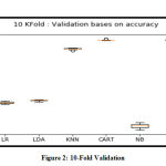Figure 2: 10-Fold Validation Click here to View Figure

 

Comparative Analysis

An analysis of contemporary work in this context shows that most of the authors are focusing on using combination feature selection approaches. The authors³⁶ are using fluorescence and spectral- morphological features to train a neural network. With six class datasets, they were able to achieve an average accuracy of 95.5 %. The authors³⁷ have also worked on identification of freshwater algae. These authors are also using a combination of PCA and neural network for training the feature data. The feature data consists of text and shape properties of six algae species and the average accuracy achieved is close to 95.9%. There is evidence in the current literature ³⁸ that neural network modeling architecture has also been used. The authors ³⁸ were able to identify four algae with the help of a feed forward model, and were able to achieve  95-97% average accuracy in classification and identification of these algae species. The outcome produced here worked for all ten types of microorganisms. The accuracy level (98 %) of the CART algorithm can be attributed to the fact that it has an inbuilt mechanism to handle unbalanced datasets. The CART Algorithm is able to build a generalized model and is doing its own attribute analysis to arrive at accurate classification, which is a great advantage. The SVC uses One-vs.-One strategy to classify the data into ten classes of Algae. Further, it seems that LR and LDA algorithms are unable to fit data to the maximum possible level.

Conclusion

This is a real-life study, in which the collection of water samples from Sukhna and Dhanas Lakes, India has been done. Identification of 10 algae has been done with the help of experts. A good understanding of the population characteristics of algae is crucial for the ecological balance. The automation of the process of identification of the algae is need of the hour, because in the current era we are facing both man-made and natural ecological imbalances. There are multiple approaches in automating the process of identification. After conducting this empirical study, it was found that a combination approach in the segmentation of the algae works well. It was found that Otsu clustering along with Kirsch filter is most suited for segmenting the microbes. Extensive Feature analysis for building machine learning dataset has been done. Correlation as a tool for feature selection was found to be an excellent choice for eliminating variables that are having multi-collinearity. It was found that at a correlation level of 0.85, the selected features provide stable and consistent results in terms of recall, precision, and accuracy for machine learning algorithms. Experimental evaluation and study of classification algorithms showed that CART Algorithm is best suited for this purpose. The kingdom of Algae is large and diverse. In this research, we were able to cover ten types of algae. The source code and output of the segmentation algorithm for this research work is available at mendeley data repository³⁹. Hence, this work can be extended by adding more types of species and microorganisms types. The size of the dataset can also be increased and augmented with more images and annotated data. An extended system of this research may also take advantage of deep learning algorithms.

Acknowledgement

Authors are highly thankful to Dr. Sanjay Bhatia, P.G. Department of Zoology, University of Jammu, India for helping us in doing the tedious work of manual identification of microorganisms and for providing constant guidance and support.

Conflict of Interest

There is no conflict of interest.

Funding Source

The authors received no funding for this work.

References

1. Jayan H, Pu H, Sun DW. Recent development in rapid detection techniques for microorganism activities in food matrices using bio-recognition: A review. Trends Food Sci Technol. 2020;95:233-246. doi:10.1016/j.tifs.2019.11.007
   CrossRef
2. Newton RJ, McClary JS. The flux and impact of wastewater infrastructure microorganisms on human and ecosystem health. Curr Opin Biotechnol. 2019;57:145-150. doi:10.1016/j.copbio.2019.03.015
   CrossRef
3. Bellinger EG, Sigee DC. Freshwater Algae: Identification, Enumeration and Use as Bioindicators: Second Edition.; 2015. doi:10.1002/9781118917152
   CrossRef
4. Romaní AM, Chauvet E, Febria C, et al. The Biota of Intermittent Rivers and Ephemeral Streams: Prokaryotes, Fungi, and Protozoans. In: Intermittent Rivers and Ephemeral Streams: Ecology and Management. ; 2017:161-188. doi:10.1016/B978-0-12-803835-2.00009-7
   CrossRef
5. Callieri C, Eckert EM, Di Cesare A, Bertoni F. Microbial communities. In: Encyclopedia of Ecology. ; 2018. doi:10.1016/B978-0-12-409548-9.11222-9
   CrossRef
6. Kaur R, Garg V, Kaur R, Pandit S, Attri SV, Ahluwalia AS. Assessment of water quality, heavy metal contamination and its indexing approach of Dhanas Lake in Patiala Ki Rao reserved forest area, Chandigarh. Indian J Environ Prot. 2018;38(9):751-758.
7. Nong X, Shao D, Zhong H, Liang J. Evaluation of water quality in the South-to-North Water Diversion Project of China using the water quality index (WQI) method. Water Res. 2020;178. doi:10.1016/j.watres.2020.115781
   CrossRef
8. Cerone A, Scotti M. Research challenges in modelling ecosystems. In: Lecture Notes in Computer Science (Including Subseries Lecture Notes in Artificial Intelligence and Lecture Notes in Bioinformatics). ; 2015;8938. doi:10.1007/978-3-319-15201-1_18
   CrossRef
9. Pimm SL, Alibhai S, Bergl R, et al. Emerging Technologies to Conserve Biodiversity. Trends Ecol Evol. 2015;30(11):685-696. doi:10.1016/j.tree.2015.08.008
   CrossRef
10. Deans AR, Yoder MJ, Balhoff JP. Time to change how we describe biodiversity. Trends Ecol Evol. 2012;27(2):78-84. doi:10.1016/j.tree.2011.11.007
    CrossRef
11. Li C, Shirahama K, Grzegorzek M. Environmental microbiology aided by content-based image analysis. Pattern Anal Appl. 2016;19(2):531-547. doi:10.1007/s10044-015-0498-7
    CrossRef
12. Li C, Wang K, Xu N. A survey for the applications of content-based microscopic image analysis in microorganism classification domains. Artif Intell Rev. 2017:1-70. doi:10.1007/s10462-017-9572-4
    CrossRef
13. James Lani. Correlation (Pearson, Kendall, Spearman). Statistics Solutions.
14. Harrison PA, Berry PM, Simpson G, et al. Linkages between biodiversity attributes and ecosystem services: A systematic review. Ecosyst Serv. 2014;9:191-203. doi:10.1016/j.ecoser.2014.05.006
    CrossRef
15. Coltelli P, Barsanti L, Evangelista V, Gualtieri P. Algae through the looking glass. Microsc Res Tech. 2017;80(5). doi:10.1002/jemt.22820
    CrossRef
16. Sonak A, Patankar RA. A Survey on Methods to Handle Imbalance Dataset. Int J Comput Sci Mob Comput. 2015;4(11):338-343.
17. Singh DK, Singh N. Drying Urban lakes: A consequence of climate change, urbanization or other anthropogenic causes? An insight from northern India. Lakes Reserv Res Manag. 2019;24(2):115-126. doi:10.1111/lre.12262
    CrossRef
18. Chaudhry P, Sharma MP, Bhargava R. Benefit-cost analysis of lake conservation with emphasis on aesthetics in developing countries. Int J Hydrol Sci Technol. 2013;3(2):111-127. doi:10.1504/IJHST.2013.057624
    CrossRef
19. Dreiseitl S, Ohno-Machado L. Logistic regression and artificial neural network classification models: A methodology review. J Biomed Inform. 2002;35:352-359. doi:10.1016/S1532-0464(03)00034-0
    CrossRef
20. Christodoulou E, Ma J, Collins GS, Steyerberg EW, Verbakel JY, Van Calster B. A systematic review shows no performance benefit of machine learning over logistic regression for clinical prediction models. J Clin Epidemiol. 2019;110:12-22. doi:10.1016/j.jclinepi.2019.02.004
    CrossRef
21. Gilpin LH, Bau D, Yuan BZ, Bajwa A, Specter M, Kagal L. Explaining explanations: An overview of interpretability of machine learning. In: Proceedings – 2018 IEEE 5th International Conference on Data Science and Advanced Analytics, DSAA 2018. ; 2019. doi:10.1109/DSAA.2018.00018
    CrossRef
22. Holmes G, Donkin A, Witten IH. WEKA: A machine learning workbench. In: Australian and New Zealand Conference on Intelligent Information Systems – Proceedings. ; 1994. doi:10.1109/anziis.1994.396988
    CrossRef
23. Neunhoeffer M, Sternberg S. How cross-validation can go wrong and what to do about it. Polit Anal. 2019;27(1):101-106. doi:10.1017/pan.2018.39
    CrossRef
24. Hjorth JSU, Hjorth JSU. Cross validation. In: Computer Intensive Statistical Methods. ; 2018. doi:10.1201/9781315140056-3
    CrossRef
25. James B, Yoshua B. Random Search for Hyper-Parameter Optimization. J Mach Learn Res. 2012;13:281-305. doi:10.1162/153244303322533223
    CrossRef
26. Dhanachandra N, Chanu YJ. A Survey on Image Segmentation Methods using Clustering Techniques. Eur J Eng Res Sci. 2017;2(1):15. doi:10.24018/ejers.2017.2.1.237
    CrossRef
27. Guo SQ, Wang LQ, Fan HH. An image segmentation method for eliminating illumination inuence. J Inf Hiding Multimed Signal Process. 2016;7(5):1100-1109.
28. Goh TY, Basah SN, Yazid H, Aziz Safar MJ, Ahmad Saad FS. Performance analysis of image thresholding: Otsu technique. Meas J Int Meas Confed. 2018;114:298-307. doi:10.1016/j.measurement.2017.09.052
    CrossRef
29. Poudel RPK, Liwicki S, Cipolla R. Fast-SCNN: Fast semantic segmentation network. In: 30th British Machine Vision Conference 2019, BMVC 2019. ; 2020.
30. Chin CL, Wu GR, Weng TC, Kang YY, Lin BJ, Chen HF. Skin condition detection of smartphone face image using multi-feature decision method. In: Proceedings – 2017 IEEE 8th International Conference on Awareness Science and Technology, ICAST 2017. ; 2017. doi:10.1109/ICAwST.2017.8256483
    CrossRef
31. Deokate ST, Uke NJ. Hybrid methods for Segmenting and Identifying the Marathi Text. In: 2019 IEEE 5th International Conference for Convergence in Technology, I2CT 2019. ; 2019. doi:10.1109/I2CT45611.2019.9033923
    CrossRef
32. Wang C, Liu J, Chen Y, Xie L, Liu HB, Lu S. RF-Kinect: A Wearable RFID-based Approach Towards 3D Body Movement Tracking. Proc ACM Interactive, Mobile, Wearable Ubiquitous Technol. 2018;2(1). doi:10.1145/3191773
    CrossRef
33. Muhimmah I, Lusiyana N, Fatmawati. Identifying Morphology of the Rat Flea Arthropod as a Vector of Plague Disease Based Microscopic Image. In: IOP Conference Series: Materials Science and Engineering. ; 2020;722. doi:10.1088/1757-899X/722/1/012065
    CrossRef
34. Elseid AAG, Hamza AOM. Computer-Aided Glaucoma Diagnosis System. 1^st ed. 2020. doi:10.1201/9780367406288
    CrossRef
35. Khaire UM, Dhanalakshmi R. Stability of feature selection algorithm: A review. J King Saud Univ – Comput Inf Sci. 2019. doi:10.1016/j.jksuci.2019.06.012
    CrossRef
36. Deglint JL, Jin C, Wong A. Investigating the Automatic Classification of Algae Using the Spectral and Morphological Characteristics via Deep Residual Learning. In: Springer, Cham; 2019:269-280. doi:10.1007/978-3-030-27272-2_23
    CrossRef
37. A. Victoria Anand Mary GP and SM. Freshwater Microalage Image Identification and Classification Based on Machine Learning Technique. Asian J Comput Sci Technol. 2018;7(1):63-67.
38. J.L. Deglint, C. Jin AC and AW. The Feasibility of Automated Identification of Six Algae Types Using Feed-Forward Neural Networks and Fluorescence-Based Spectral-Morphological Features. IEEE Access. 2019;7:7041–7053.
    CrossRef
39. Dhindsa A, Bhatia S, Agrawal S., Sohi B.S. Dataset for Efficient Microbes Detection System using Microscopic Images via Morphological and Correlation Based Features. 2020; Mendeley Data,v2. doi: 10.17632/f9m85ptmvc.2
    CrossRef

(Visited 617 times, 1 visits today)