Alpika Tripathi^1*, Geetika Srivastava², K.K. Singh³ and P.K. Maurya⁴

¹Department of Computer Science and Engineering, ASET, Amity University, Lucknow - 226010, India.

²Department of Physics and Electronics, Dr. RML Avadh University, Faizabad - 224001, India.

³Department of E and CE, ASET, Amity University, Lucknow - 226010, India.

⁴Department of Neurology, RML Institute of Medical Sciences, Lucknow - 226010, India.

Corresponding Author E-mail: alpika2k@gmail.com

DOI : https://dx.doi.org/10.13005/bpj/1674

Abstract

The objective of this paper is to make a distinction between EEG data of normal and epileptic subjects. Methods: The dataset is taken from 20-30 years healthy male/female subjects from EEG lab of Dept. of Neurology, Dr. RML Institute of Medical Sciences, Lucknow (India). The feature extraction has been done using the Hilbert Huang Transform (HHT) method. The experimental EEG signals have been decomposed till 5th level of Intrinsic Mode Function (IMF) followed by calculation of high order statistical values of each IMF. Relief algorithm (RBAs) is used for feature selection and classification is performed using Linear Support Vector Machine (Linear SVM). This paper gives an independent approach of classifying Epileptic EEG data with reduced computational cost and high accuracy. Our classification result shows sensitivity, specificity, selectiv­ity and accuracy of 96.4%, 79.16%, 84.3% and 88.5% respectively. The proposed method has been analyzed to be very effective in accurate classification of epileptic EEG data with high sensitivity.

Keywords

Epilepsy; EEG; Hilbert Huang Transform (HHT); Relief-Based Feature Selection Algorithms (Rbas); Linear Support Vector Machine (SVM)

Download this article as: 

Copy the following to cite this article: Tripathi A, Srivastava G, Singh K. K, Maurya P. K. Epileptic Seizure Data Classification Using RBAs and Linear SVM. Biomed Pharmacol J 2019;12(2).

Copy the following to cite this URL: Tripathi A, Srivastava G, Singh K. K, Maurya P. K. Epileptic Seizure Data Classification Using RBAs and Linear SVM. Biomed Pharmacol J 2019;12(2). Available from: https://bit.ly/2IMPKZs

Introduction

PILEPSY is a physical condition that occurs in the brain and affects the nervous system. According to the 2009 report by the World Health Organization around 70 million people worldwide have epilepsy.^1-3 Around 90% of this population lives in developing countries, and about three fourths of them do not have access to the necessary treatment. Epilepsy is defined by two or more such unprovoked seizures.⁴ The seizures are commonly defined as abnormal electrical and chemical activities in the brain. Like many other neurological disorders, epilepsy can be assessed by the electroencephalogram (EEG). The EEG signal is highly non-linear and non-stationary in nature, and hence, it is difficult to characterize and interpret it using conventional frequency domain analysis.^5-7

EEG is recording of the electrical activity of the brain from the scalp. The recorded waveforms reflect the cortical electrical activity and helps in identification of brain conditions. The most common method used for recording EEG is 10-20 system which is internationally recognized method that allows EEG electrode placement to be standardized.⁸

The system is based on the relationship between the location of an electrode and the underlying area of outer layer of the brain. The number ‘10’ & ‘20’ refer to the distance between adjacent electrode to be either 10% or 20% of the total front-back or right-left distance of the scalp . The electrode placement is shown in Figure 1.

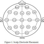Figure 1: Scalp Electrode Placement.   Click here to view figure

 

In this paper authors have given a method for classification of epileptic and normal EEG data. The proposed method uses a combination of Hilbert Huang Transform (HHT) for features extraction, RBAs for feature selection and Linear SVM based classification of neural network modeling.

Hilbert-Huang Transform is a time frequency technique consisting of two parts, the Empirical Mode Decomposition (EMD), and the Hilbert Spectral Analysis (HSA).^9,10 EMD decomposes an EEG signal into a finite set of band-limited signals termed intrinsic mode functions (IMFs), which are oscillatory components of input data. In the first step the mean frequency (MF) for each IMF has been computed using Fourier-Bessel expansion.¹¹ The IMF oscillates in a narrow frequency band which is a reflection of quasi-periodicity and nonlinearity. The non-constant frequency means non-stationary. MF measure of the IMFs has been used as one of the features to differentiate between healthy and epileptic EEG signals. In the second part, the Hilbert transform is applied to the IMF, yielding a time-frequency representation (Hilbert spectrum) for each IMF.^12,13

For feature selection authors have used Relief algorithm.^14-17 Relief is an algorithm in which a filter-method approach is used for feature selection that is notably sensitive to feature interactions. It was originally designed for application to binary classification problems with discrete or numerical features. Relief was also described as generalizable to polynomial classification by decomposition into a number of binary problems.

Relief calculates a feature score for each feature which can then be applied to rank and select top scoring features for feature reduction. Alternatively, these scores may be applied as feature weights to guide downstream modeling. Relief feature scoring is based on the identification of feature value differences between nearest neighbor instance pairs. If a feature value difference is observed in a neighboring instance pair with the same class (a ‘hit’), the feature score decreases. Alternatively, if a feature value difference is observed in a neighboring instance pair with different class values (a ‘miss’), the feature score increases shown in Figure 2.

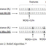Figure 2: Relief Algorithm.14   Click here to view figure

 

The Support Vector Machine (SVM) is a popular classifier that can handle linear as well as non-linear class boundaries with the help of kernel functions.¹⁸ In this paper authors have used Linear SVM for data classification. The SVM tries to identify the maximum-margin hyper plane that separates the different classes. However, if the data cannot be linearly separated, non-linear kernel functions are used to transform the feature space, allowing a maximum-margin hyper plane to be established.¹⁹

HHT based feature extraction

The Hilbert–Huang transform (HHT) is an empirical data-analysis method. Its basis of expansion is adaptive, so it produces physically meaningful representations of data from nonlinear and non-stationary processes.^20,21 Traditional data-analysis methods are all based on linear and stationary assumptions like Fourier transformation makes assumption of the signal period which creates spectral leakage. As is well known, the natural physical processes are mostly nonlinear and non-stationary like EEG signals from brain, yet the conventional data analysis methods provide very limited options for examining data from such processes. The available methods are either for linear but non-stationary, or nonlinear but stationary and statistically deterministic processes.

It is known that frequency of sinusoidal waveform is a well defined quantity. However, in practice, signals are not purely sinusoidal or stationary. Thus representing such non stationary signals as combination of different sinusoidal components will be a compromise with the accurate assessment of an event. For such signal the term frequency loses its effectiveness and a need for a parameter which accounts for the varying nature of the phenomena arises.

This gives rise to an idea of instantaneous frequency (IF) – which means the signal is either composed of a single frequency or a narrow band of frequencies. For each component instantaneous frequency can be defined.

HHT was motivated by the need to describe nonlinear distorted waves in detail, along with the variations of these signals that naturally occur in non-stationary processes.

The empirical mode decomposition method is necessary to deal with data from non-stationary and nonlinear processes.^22,23 EMD decomposes signal X (𝑡) into a number of oscillatory component which is known as intrinsic mode function through a shifting process. Each IMF has its own distinct time scale. Furthermore EMD does not consider the stationary and the linearity of the signal.²⁰ For an input signal X (𝑡) the process of calculating IMFs are given below:

Let’s set

X(𝑡) = X(𝑡)_𝑜𝑙𝑑………………………… (1)

Find all the maxima and minima in

X(𝑡)_𝑜𝑙d…………………………………(2)

Interpolate between minima and maxima using cubic spline interpolation which will generate local maxima envelope (𝑡) and local minima envelope

𝑒l(𝑡)…………..…………………………(3)

Calculate the mean of envelopes

𝑒𝑚𝑒𝑎𝑛 = ((𝑡)+𝑒𝑙(𝑡))/2………………….(4)

Now subtract 𝑒𝑚𝑒𝑎𝑛 from X(𝑡)_𝑜𝑙𝑑 we will get X(𝑡)_𝑛𝑒𝑤as,

X(𝑡)_𝑛𝑒𝑤 = X(𝑡)_𝑜𝑙𝑑 –𝑒𝑚𝑒𝑎𝑛……….,………(5)

Now set

X(𝑡)_𝑜𝑙𝑑 = X(𝑡)_𝑛𝑒𝑤 ……………..………..(6)

Repeat the process (2 to 4) until standard deviation

SD = (∑│X(t)_new –X(t)_old │² / ∑ X(t)²_old ) < α…..(7)

Where α is value that between 0.2-0.3

The first IMF is defined as IMF1 = X(𝑡)_𝑛𝑒𝑤 which is the smallest temporal scale of X(𝑡). By subtracting IMF1 from X(𝑡) we will get residual signal R(𝑡) which can be expressed as ,

R(𝑡) = X(𝑡) – IMF1.

After acquiring R(𝑡) we put it in the same process above to get new IMF which means each IMF will have different frequencies against time. So the original signal can be rewritten as

Hilbert Huang Transform (HHT) is a very new and powerful tool for analyzing data from non-stationary and nonlinear processing realm and capable of filtering data based on empirical mode decomposition (EMD). The EMD is based on the sequential extraction of energy associated with various intrinsic time scales of the signal; therefore total sum of the intrinsic mode functions (IMFs) matches the signal very well and ensures completeness.

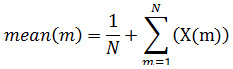
Studies show that we can discriminate between normal EEG data and abnormal EEG by statistically analyzing the IMF. Their statistical use is motivated by the fact that the distributions of samples in the data are characterized by their asymmetry, dispersion and concentration around the mean. After analyzing visually we can see IMF obtained from normal and pathological EEG are quite different from one another. These differences can easily extracted by statistical methods like Mean Function (MF), Standard Deviation (SD), Variance (VAR), Kurtosis (KUR), Skewness (SKW).^24-26

Mean: Computes the average values of the signal at various frequency levels.

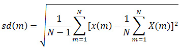
Standard Deviation: For calculating the variations of signal at various levels.

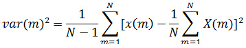
Variance: It is the square of the standard deviation.

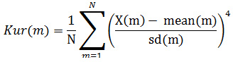
Kurtosis: Coefficients of EEG signal do not follow the normal distribution, and have a heavy tail characteristic is justified by the value of kurtosis parameters.

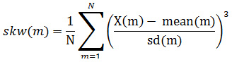
Skewness: It is a measure of the asymmetry. If the probability distribution of a real-valued random variable around its mean is not symmetrical, the data is said to be skewed.

The same processing steps are further applied on other 16 channels of EEG recording of Normal and Epileptic subjects.

Relief Based Feature Selection Algorithm

Take a data set with n instances of p features, belonging to two known classes. Within the data set, each feature should be scaled to the interval [0 1] (binary data should remain as 0 and 1). The algorithm will be repeated k times. Start with a p-long weight vector (G) of zeros.

At each iteration, take the feature vector (V) belonging to one random instance, and the feature vectors of the instance closest to V (by Euclidean distance) from each class. The closest same-class instance is called ‘near-hit’, and the closest different-class instance is called ‘near-miss’. Update the weight vector such that

G_i = G_i – (v_i – nearHit_i)² + (v_i – nearMiss_i)²

Thus the weight of any given feature decreases if it differs from that feature in nearby instances of the same class more than nearby instances of the other class, and increases in the reverse case.

After k iterations, divide each element of the weight vector by k. This becomes the relevance vector. Features are selected if their relevance is greater than a threshold T.

Kira and Rendell’s experiments showed a clear contrast between relevant and irrelevant features, allowing T to be determined by inspection.²⁷ However, it can also be determined by Chebyshev’s inequality for a given confidence level (α) that a T of 1/sqrt(α*k) is good enough to make the probability of a Type I error less than α, although it is stated that T can be much smaller than that.

Classification using Linear SVM

Support Vector Machine (SVM) is a supervised machine learning algorithm which can be used for both classification and regression based problems. However, it is mostly used in classification problems. In this algorithm, we plot each data item as a point in n-dimensional space (where n is number of features you have) with the value of each feature being the value of a particular coordinate. Then, we perform classification by finding the hyper-plane that differentiate the two classes very well (look at the below snapshot) shown in Figure 3[A].

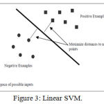Figure 3: Linear SVM.   Click here to view figure

 

Support Vectors are simply the co-ordinates of individual observation. Support Vector Machine is a frontier which best segregates the two classes (hyper-plane/ line).²⁴ In the linear case, the margin is defined by the distance of the hyper plane to the nearest of the positive and negative examples. The formula for the output of a linear SVM is

v = ѡ̄ * xˉ – b (1)

where w is the normal vector to the hyper plane and x is the input vector. The separating hyper plane is the plane v=0. The nearest points lie on the planes v = ±1. The margin m is thus

k = 1/║ѡ║₂

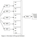Figure 4: Flowchart of Proposed Method.   Click here to view figure

 

Result and Discussion

This paper gives the feature extraction results produced by applying decomposition of signal till fifth level of IMFs by applying HHT on EEG signals, and then RBA is used for feature selection, followed by Linear SVM for classification. The normal and abnormal input data is applied after removing artifacts.

Statistical values of 29 EEG signals of normal subjects upto 5^th IMF has been shown in table 1 and values of 23 EEG signal of Epileptic subjects has been displayed in table 2. On the basis of these obtained values, the training and testing of Linear SVM classifier has been proposed. 70% of data set is used for training purpose and rest 30% were utilised for testing results.

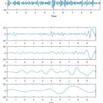Figure 5: IMFs of Normal EEG Signal.   Click here to view figure

 

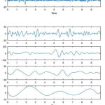Figure 6: IMFs of Epileptic EEG Signal.   Click here to view figure

 

Once the calculation of IMFs is complete, the following important statistical parameters are evaluated. Table 1 & 2 are presenting the calculated statistical values of Healthy and Unhealthy subjects.

Table 1: High Order Statistical Values of 29 EEG signal of Normal Subjects upto 5^th IMF.

HOS Values of 29 EEG Signals	High Order Statistical Values
IMF	MF	SD	VAR	KUR	SKW
Subjects	IMF 1 of Healthy Subjects
NS1	0.794014	0.194748	0.0808656	0.0574944	0.0275939
NS2	0.7134649	0.3835633	0.1539171	0.0777196	0.0382288
NS3	0.7120425	0.392048	0.125765	0.0633654	0.0277442
NS4	0.6561924	0.3911876	0.1600673	0.0619577	0.0186501
NS5	0.7923439	0.39687	0.1419385	0.0608046	0.0248904
NS6	0.69531	0.3801633	0.1490987	0.0560318	0.0249986
NS7	0.6191468	0.3552116	0.1217889	0.0628417	0.0204335
NS8	0.6190132	0.2576959	0.1470799	0.0867544	0.0133281
NS9	0.7279635	0.3972242	0.1589645	0.0708214	0.0291047
NS10	0.6938438	0.3249872	0.1626327	0.0611141	0.0319724
NS11	0.6037114	0.2716271	0.1364642	0.0631772	0.0158963
NS12	0.5959096	0.2387053	0.1123194	0.0494584	0.0204792
NS13	0.7039527	0.3296545	0.1480881	0.0748475	0.0269281
NS14	0.6844529	0.4312466	0.165582	0.0781406	0.0422987
NS15	0.7843782	0.4633051	0.1519389	0.0567255	0.0207948
NS16	0.7207146	0.356144	0.1542686	0.0732491	0.023715
NS17	0.7776593	0.4194125	0.157747	0.0816223	0.0360981
NS18	0.7018462	0.4333557	0.1727692	0.0736394	0.0344944
NS19	0.7561062	0.3031047	0.1599127	0.0667163	0.0298385
NS20	0.5615601	0.2440335	0.1393101	0.0625563	0.0232113
NS21	1.0151271	0.5419102	0.2060411	0.1060046	0.0350871
NS22	0.7082527	0.4058785	0.1250664	0.061215	0.0242943
NS23	0.58942	0.2640501	0.1342691	0.0745797	0.0292519
NS24	0.6863921	0.2591281	0.1569117	0.0679083	0.0330215
NS25	0.6579692	0.3820743	0.1577376	0.0544039	0.0247068
NS27	0.6185096	0.3248713	0.1347292	0.0557921	0.0208321
NS28	0.7167416	0.2263721	0.1505363	0.0735477	0.0337342
NS29	0.4230327	0.3507278	0.1417878	0.0668265	0.026326
Subjects	IMF 2 of Healthy Subjects
NS1	1.3671451	2.8716697	6.5527059	9.3498067	8.6381729
NS2	1.1840138	1.3916471	2.8017808	2.4379485	2.2303501
NS3	0.843453	0.9167091	2.4823977	3.5295424	3.3642967
NS4	0.8421751	0.9637028	2.2007558	2.8008546	5.2072605
NS5	0.5406368	0.9089775	2.0956593	4.9641066	2.7387957
NS6	0.6736103	0.8451676	2.1182751	3.4507008	3.1589237
NS7	0.9872215	1.0550772	2.5285452	2.9370106	5.9665401
NS8	4.5190525	6.5279076	9.970391	5.4465119	20.088837
NS9	0.5998085	0.8185307	1.6512623	2.3169359	3.1302619
NS10	0.8223158	1.0699668	1.8031497	2.367291	2.5566929
NS11	1.0965751	1.460845	2.553014	2.7946504	5.9919763
NS12	1.1829003	1.7480142	3.5795746	4.8171016	4.7400878
NS13	1.0971638	1.4864917	2.6012838	2.1556349	2.5493749
NS14	0.4312608	0.5038683	0.9079241	1.3058499	1.4082351
NS15	1.5704348	1.487021	2.6870926	7.916428	14.940614
NS16	0.8077475	1.0170576	2.5210509	2.3879847	2.7999426
NS17	0.4905736	0.7537514	1.8861905	1.9574766	1.9970076
NS18	0.7166195	1.0073588	2.0143632	2.1873461	2.7866116
NS19	0.680081	1.1124491	1.9422344	2.3306878	3.7269487
NS20	3.0825562	4.1088006	5.6119314	4.6420457	3.914372
NS21	3.0527935	3.1810749	2.9614952	2.9901266	2.0240628
NS22	0.6201656	0.6909153	2.2992595	3.5640906	3.9328668
NS23	2.1344174	2.6372075	4.8936201	3.6146932	3.2462856
NS24	0.5554465	1.3915533	2.3443719	2.6064464	1.9867625
NS25	1.0111484	1.1234713	2.0467199	3.0696111	2.481803
NS27	1.1047307	1.2129053	2.3732381	3.3731465	5.2515313
NS28	0.6727835	1.6808005	3.1633969	3.2929552	2.621261
NS29	0.5791149	0.5605072	1.4387479	1.9286429	3.2353766
Subjects	IMF 3 of Healthy Subjects
NS1	1.8690857	8.246487	42.937955	87.418885	74.618031
NS2	1.4018887	1.9366815	7.8499754	5.9435931	4.9744615
NS3	0.7114129	0.8403556	6.1622985	12.45767	11.318492
NS4	0.7092588	0.928723	4.8433261	7.8447862	27.115562
NS5	0.2922881	0.8262401	4.3917878	24.642354	7.5010021
NS6	0.4537508	0.7143082	4.4870895	11.907336	9.978799
NS7	0.9746063	1.1131878	6.3935406	8.6260312	35.5996
NS8	20.421835	42.613577	99.408696	29.664492	403.56139
NS9	0.3597703	0.6699926	2.7266671	5.3681922	9.7985398
NS10	0.6762032	1.144829	3.251349	5.6040665	6.5366786
NS11	1.2024769	2.1340681	6.5178805	7.8100709	35.90378
NS12	1.399253	3.0555538	12.813354	23.204467	22.468433
NS13	1.2037684	2.2096577	6.7666774	4.6467616	6.4993125
NS14	0.1859859	0.2538833	0.8243261	1.705244	1.9831261
NS15	2.4662655	2.2112313	7.2204666	62.669832	223.22196
NS16	0.652456	1.0344061	6.3556978	5.7024708	7.8396784
NS17	0.2406624	0.5681411	3.5577147	3.8317147	3.9880392
NS18	0.5135434	1.0147717	4.0576589	4.7844829	7.7652043
NS19	0.4625101	1.237543	3.7722746	5.4321057	13.890147
NS20	9.5021525	16.882242	31.493774	21.548588	15.322308
NS21	9.3195484	10.119238	8.770454	8.940857	4.0968302
NS22	0.3846054	0.477364	5.2865944	12.702742	15.467441
NS23	4.5557378	6.9548636	23.947518	13.066007	10.53837
NS24	0.3085208	1.9364205	5.4960795	6.7935628	3.9472251
NS25	1.0224211	1.2621877	4.1890623	9.4225121	6.1593459
NS27	1.22043	1.4711394	5.6322589	11.378117	27.578581
NS28	0.4526377	2.8250902	10.00708	10.843554	6.871009
NS29	0.3353741	0.3141683	2.0699954	3.7196636	10.467662
Subjects	IMF 4 of Healthy Subjects
NS1	26.1211	173.58881	105.7402	86.502577	14.866722
NS2	4.5384237	5.8235914	3.3288413	3.9677612	3.7352665
NS3	4.4268523	6.0777767	6.4834451	4.3057737	4.129212
NS4	13.246323	6.5958737	3.7837047	3.3066044	4.5568696
NS5	5.8715379	9.3080921	4.438701	2.8511137	3.3463041
NS6	4.7410993	5.602009	3.5239203	3.5818778	3.7913422
NS7	5.019083	4.3211797	7.0526305	3.8742989	6.3995483
NS8	12.323221	26.213322	6.9748686	5.203992	14.349722
NS9	5.2998872	8.1148395	4.0907434	3.5577341	2.7479037
NS10	5.5523941	15.273256	3.2721178	4.860471	3.6195343
NS11	5.1316229	7.6528964	3.4040442	3.4681068	11.761679
NS12	24.611047	7.1365169	4.9725586	7.1197671	7.7796655
NS13	4.9092302	7.0940397	3.7071417	4.1142901	4.2781562
NS14	142.10583	27.677388	4.7715764	3.4914967	2.9643649
NS15	8.9146693	7.9038536	10.159726	7.0833235	5.5552036
NS16	7.5069103	10.522004	5.2477441	3.1655753	4.1332655
NS17	6.2864369	3.7169318	3.4123277	3.6338549	3.3516207
NS18	7.3879998	3.6279616	3.2416907	4.0381763	12.696512
NS19	124.96265	7.2477353	3.3237369	3.8798556	5.3328726
NS20	4.8953379	6.7082148	3.0854336	4.6323791	5.6055095
NS21	19.483011	18.089693	4.9513198	4.9412625	2.9780993
NS22	18.376056	6.0605848	5.1925368	7.9395411	9.4866847
NS23	4.3802035	6.3862992	3.1073743	2.9512085	8.2121815
NS24	5.8519008	7.5350298	3.1145678	3.5716336	4.0131338
NS25	4.8353898	4.4480728	3.2057832	6.4106097	4.777637
NS27	6.9280576	6.504447	5.4986645	7.9219861	13.547343
NS28	81.381915	12.772316	3.7331439	3.2206681	3.218636
NS29	859.94158	22.498134	4.7187115	4.8681671	4.070564
Subjects	IMF 5 of Healthy Subjects
NS1	0.9368617	2.2400095	1.8788759	-4.6346204	-0.4742972
NS2	-0.0641331	0.02556	0.0213764	-0.1746376	-0.1316439
NS3	-0.0329525	-0.0372348	-0.170347	0.03744	-0.2469791
NS4	0.0760672	-0.0646503	0.078916	-0.0567486	0.265975
NS5	0.1335422	-0.0651292	-0.0394491	-0.1116554	-0.5056581
NS6	-0.0182776	-0.1920655	0.0125293	-0.0639116	0.2236741
NS7	0.0518529	0.0462345	0.2674941	0.0297923	-0.7641902
NS8	0.0091883	-0.2378462	0.0179487	0.0271938	1.0651003
NS9	-0.0182481	-0.0174901	0.0300339	0.0872897	-0.0599968
NS10	-0.0801845	0.6202513	-0.0045994	0.2976808	-0.0249067
NS11	-0.039921	0.3110126	0.086128	-0.0891201	-0.345381
NS12	1.2827003	-0.0110624	-0.0726262	0.0017892	-0.6870894
NS13	0.0069424	-0.0484375	0.0417263	-0.1836737	0.3871868
NS14	-0.6105902	1.2346839	0.1682674	0.0953418	-0.0021122
NS15	-0.1261543	-0.4746706	-0.3580666	0.2197198	-0.0952142
NS16	0.0352776	0.2623286	0.0164817	0.1063452	-0.2706383
NS17	-0.0915483	0.0119703	-0.0373728	0.0496959	0.2590188
NS18	0.1835534	0.0202854	-0.0084826	0.0108377	0.9936275
NS19	4.2085615	0.0127075	-0.059354	-0.2144468	-0.2042717
NS20	-0.0086416	-0.0772461	-0.0441348	-0.0245628	0.4144225
NS21	0.1078166	0.2286214	0.0188273	0.0214265	0.000411
NS22	-0.6105868	-0.1642786	0.0458767	0.8285085	-0.2906335
NS23	0.0155542	0.1616218	0.0071227	-0.0232878	-1.1183538
NS24	-0.0677949	-0.0092523	0.0438202	-0.0172195	-0.2904886
NS25	-0.0088769	0.0240307	-0.0392672	0.3934843	0.5874376
NS27	-0.0855313	-0.0039345	-0.1527337	0.2219079	-0.7106446
NS28	-0.3867619	-0.1214849	-0.0287683	-0.0250265	-0.1046807
NS29	24.095343	-0.4350748	0.0042242	0.0465327	-0.1108155

 

Table 2: High Order Statistical Values of 23 EEG signal of Epileptic Subjects upto 5^th IMF.

HOS Values of 23 EEG Signals	High Order Statistical Values
IMF	MF	SD	VAR	KUR	SKW
Subjects	IMF 1 of Unhealthy Subjects
ES1	0.8650899	0.4729091	0.0656301	0.0500698	0.0282743
ES2	0.7204698	0.301023	0.1401935	0.0650751	0.0277056
ES3	0.8391117	0.5123799	0.1675866	0.0580672	0.017728
ES4	0.6846268	0.2982419	0.1178403	0.0341233	0.019428
ES5	0.8246545	0.5175436	0.1532076	0.0706868	0.037721
ES6	0.7866724	0.5715599	0.1436699	0.0708974	0.0364508
ES7	0.7180737	0.5269248	0.1003643	0.0498809	0.0373853
ES8	0.6780945	0.2309114	0.1450357	0.0151319	0.0131524
ES9	0.6633649	0.2670126	0.1298747	0.0509755	0.029085
ES10	0.6764995	0.3393412	0.1618375	0.0640588	0.0253861
ES11	0.8552998	0.4695551	0.1592763	0.0396773	0.0178348
ES12	0.9608706	0.3980764	0.1618239	0.0526249	0.0202914
ES13	0.6468634	0.2672435	0.1478045	0.0621515	0.0111755
ES14	0.7191737	0.4133107	0.1478768	0.0643535	0.0182317
ES15	0.5935737	0.261775	0.1387919	0.0708448	0.0263439
ES16	0.7620866	0.2757785	0.0989844	0.0334673	0.0162968
ES17	0.6647294	0.3585806	0.1565834	0.0678156	0.0250318
ES18	0.7578168	0.4157828	0.1355068	0.0425817	0.0257703
ES19	0.8166415	0.4948268	0.09664	0.0278963	0.0233678
ES20	0.6549819	0.2668567	0.1455575	0.0675608	0.0255792
ES21	0.6143616	0.4561768	0.1217524	0.0705827	0.0390815
ES22	0.8869436	0.0897994	0.089129	0.0387991	0.0219594
ES23	0.9041045	0.5533729	0.1935902	0.0959522	0.0479147
Subjects	IMF 2 of Unhealthy Subjects
ES1	0.3303539	0.4068024	5.0004128	6.9876397	4.450579
ES2	0.7759541	1.1785239	2.2471837	2.6743979	2.9395671
ES3	0.9123532	1.0098045	1.2550563	2.205777	10.381173
ES4	0.4983477	0.9938214	3.0678322	10.58149	16.008316
ES5	0.3640596	0.4457771	1.0317171	1.9604556	2.8770458
ES6	0.4965187	0.7479746	1.5959717	2.2057836	2.4487858
ES7	0.4709187	0.4566298	1.689656	4.7747918	3.8819404
ES8	2.2989287	2.7078515	4.1221566	13.077719	19.783741
ES9	0.5902094	1.0359951	1.9711336	4.1579259	5.7722332
ES10	1.1322866	1.3598762	2.584256	3.8131407	4.8031704
ES11	0.7589179	0.8662426	1.49653	4.2199104	6.6306221
ES12	0.4402255	0.4632958	0.8848784	2.8468135	5.2325725
ES13	2.1736135	2.5147764	5.2851702	3.4996659	13.125115
ES14	0.5805407	0.6980601	1.8219706	2.5253038	11.036471
ES15	2.2502876	2.9015059	4.0772807	3.3953816	2.7857397
ES16	0.3805414	0.7496236	3.5402665	12.479548	12.62304
ES17	1.0604954	1.1549985	2.0075533	2.6702119	5.2474406
ES18	0.5168601	0.6714232	1.6591487	6.2580204	5.0768957
ES19	0.5728281	0.5966072	1.6938629	6.5959014	7.3144355
ES20	1.3439738	2.0153848	3.1818819	2.2977474	2.7072257
ES21	0.3307135	0.4728326	1.7315057	2.1334664	2.3625637
ES22	0.3404253	2.8266346	2.919212	6.7144357	7.7731332
ES23	1.0936969	1.0679932	1.7261892	1.9150612	1.8657758
Subjects	IMF 3 of Unhealthy Subjects
ES1	0.1091337	0.1654882	25.004129	48.827109	19.807653
ES2	0.6021047	1.3889186	5.0498348	7.1524041	8.6410547
ES3	0.8323884	1.0197052	1.5751663	4.8654523	107.76876
ES4	0.2483504	0.987681	9.4115946	111.96793	256.26619
ES5	0.1325394	0.1987172	1.0644402	3.8433861	8.2773925
ES6	0.2465308	0.5594661	2.5471256	4.8654812	5.9965518
ES7	0.2217644	0.2085108	2.8549373	22.798637	15.069461
ES8	5.2850734	7.3324599	16.992175	171.02673	391.39639
ES9	0.3483471	1.0732858	3.8853676	17.288348	33.318676
ES10	1.2820729	1.8492632	6.6783789	14.540042	23.070446
ES11	0.5759564	0.7503762	2.239602	17.807644	43.965149
ES12	0.1937985	0.214643	0.7830098	8.104347	27.379815
ES13	4.7245957	6.3241006	27.933024	12.247662	172.26864
ES14	0.3370275	0.4872879	3.3195768	6.3771594	121.8037
ES15	5.0637941	8.4187365	16.624218	11.528616	7.7603459
ES16	0.1448118	0.5619355	12.533487	155.73913	159.34114
ES17	1.1246505	1.3340216	4.0302702	7.1300316	27.535632
ES18	0.2671444	0.4508091	2.7527745	39.162819	25.77487
ES19	0.328132	0.3559401	2.8691715	43.505915	53.500966
ES20	1.8062657	4.0617758	10.124372	5.2796432	7.3290711
ES21	0.1093714	0.2235707	2.998112	4.5516789	5.5817073
ES22	0.1158894	7.9898633	8.5217987	45.083647	60.4216
ES23	1.1961729	1.1406094	2.9797292	3.6674596	3.4811194
Subjects	IMF 4 of Unhealthy Subjects
ES1	4.5771176	7.0087635	18.72618	4.438525	3.6387834
ES2	4.6721191	12.485297	3.7515448	2.8945809	3.2989253
ES3	4.8363808	3.6414101	4.8090367	9.1757919	3.8358201
ES4	25.708015	29.801328	6.3511609	12.355667	2.2715564
ES5	8.4152284	3.0111605	5.1884963	11.195804	4.1664795
ES6	8.058631	2.5071926	5.6127706	4.8551599	3.3116094
ES7	294.40981	3.1362269	27.83137	5.3359899	2.957612
ES8	4.9401601	11.098406	3.3255404	35.553052	18.566356
ES9	14.952852	13.619801	5.7570903	8.0806325	12.965434
ES10	4.5372324	6.8736788	3.6542007	6.0117279	12.628416
ES11	3.7915257	3.8012139	5.0176857	10.534601	16.394638
ES12	8.3659199	66.930757	9.4311181	14.648822	13.724967
ES13	7.3759178	12.338818	2.9419575	21.578049	31.927595
ES14	63.38271	4.2477574	3.713664	5.0928349	8.7693387
ES15	6.158873	5.8291961	3.826798	2.9856206	4.9684164
ES16	43.596893	24.808282	5.9428689	5.6386731	7.2970514
ES17	5.4453413	6.0432796	3.93111	6.0310116	7.4071691
ES18	17.473343	7.0504811	4.7559268	4.5921542	3.0711551
ES19	223.20771	6.1305469	30.525167	43.536547	22.863897
ES20	3.83648	6.6480955	3.4461044	3.1125352	3.3795001
ES21	395.02359	7.7392785	15.905384	5.0630354	3.1100875
ES22	6.965067	100.63262	22.440095	16.072997	8.0500811
ES23	4.7254519	4.026748	6.3249347	10.183007	15.691209
Subjects	IMF 5 of Unhealthy Subjects
ES1	0.024654	-0.4296459	0.3575977	0.0226011	-0.0755703
ES2	0.0061941	0.5499125	-0.1601651	0.0755629	0.1800178
ES3	0.0010872	-0.0197224	-0.0789725	-0.140138	0.1755386
ES4	-0.7393064	-0.4796606	-0.0979807	-0.8759199	0.090423
ES5	0.2707581	-0.001205	-0.0570468	0.2302964	0.2013605
ES6	-0.0974631	0.0032945	0.0368402	-0.1686396	0.1249878
ES7	9.9175498	0.0201692	-2.417516	-0.1451854	0.0458859
ES8	0.0410811	-0.3725798	0.0468306	-3.5959749	1.6056099
ES9	-0.7679569	-0.2677045	-0.2248263	0.1450071	0.2373168
ES10	0.011263	0.2940156	0.0009562	0.3756074	0.2475115
ES11	-0.0123112	0.0664354	-0.103722	1.323574	2.3883766
ES12	0.3587948	-1.3089528	-0.3568748	0.9671277	-1.8264115
ES13	0.352495	0.236305	-0.00324	-2.3182493	-4.0947717
ES14	-2.6589605	0.0485656	0.0581806	-0.0709458	-0.0135256
ES15	0.1221658	0.0747326	0.0272607	0.0547411	-0.2824818
ES16	-2.2468663	0.0203399	0.0164117	0.0324535	-0.9939975
ES17	0.076271	-0.1215204	0.1040614	-0.059463	-0.3068512
ES18	0.9846622	-0.0624885	0.0260383	0.1778707	-0.0116882
ES19	6.9752414	-0.1316119	-0.0018436	-3.9574945	-1.6565017
ES20	-0.0276649	-0.1214705	-0.0007395	0.0384048	-0.0818361
ES21	14.24066	0.1333398	-0.3670489	0.0921567	-0.0049415
ES22	0.2247009	-3.5664924	-0.315258	0.7120273	-0.5549812
ES23	-0.0670528	-0.0564401	-0.0320062	-0.5541185	-1.4992487

 

For feature selection Relief algorithm calculates a feature score for each feature which can then be applied to rank and select top scoring features. The Hilbert–Huang transform (HHT) is a way to decompose a signal into intrinsic mode functions (IMF) along with a trend, and obtain instantaneous frequency data and used for feature extraction. For classifying the experimental EEG signals, the Linear SVM concept has been used. The computed statistical values are fed into Linear SVM classifier for training and testing. The performance of proposed methodology is evaluated in terms of parameters of confusion matrix & ROC Curve shown in Figure 7 & 8.

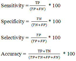
Where TP, TN, FP and FN stands for true positive, true negative, false positive and false negative respectively. Sensitivity is used to diagnose the correctly identified positive case, specificity is defined as the determination of negative cases accurately, selectivity is defined as the recognition of unidentified positive results and accuracy stands for the identification of correct classified instances.

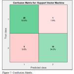Figure 7: Confusion Matrix.   Click here to view figure

 

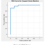Figure 8: ROC Curve.   Click here to view figure

 

Table 3: Shows the proposed classifier output and compare with existing techniques

Authors	Sensitivity	Selectivity	Accuracy
Syed Muhammad Usman et al., (2017)	92.3%	–	–
Yildiz, Bergil & C.Oral (2017)	88.06%	–	–
Bandarabadi, Mojtaba et al., (2015)	75.8%	–	–
Our Findings	96.5%	84.8%	88.5%

 

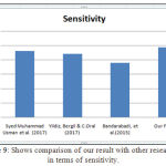Figure 9: Shows comparison of our result with other researchers in terms of sensitivity.   Click here to view figure

 

Conclusion

The proposed method is suitable for separating normal and epileptic EEG data. The com­bined approach of HHT, RBAs with Linear SVM has found to be very effective in such classification with high sensitivity. The result of the classification pro­cess is based on using the statistical values obtained by HHT. This technique has been found to be suitable in the correct classification of epileptic and healthy EEG data. The data set is taken from Natus NeuroWorks EEG Recording Machine from RML Institute of Medical Sciences, Lucknow (U.P.), India. Our classification result shows sensitivity, selectiv­ity and accuracy are 96.5%, 84.8% and 88.5% respectively.

Acknowledgements

The authors acknowledge Dr. A. K. Thacker, Head of Department, Department of Neurology, RMLIMS, Lucknow (U.P) for his valuable help in developing an understanding towards the Epilepsy. His contributions and work in the related field helped us to think a stage ahead and Ms. Nidhi, Technical Staff EEG Lab, RMLIMS, Lucknow (U.P) for providing EEG Recording of Healthy& Unhealthy Subjects.

Conflict of Interest

There is no conflict of interest.

References

1. Fisher, W. van Emde Boas, W. Blume, C. Elger, P. Genton, P. Lee, J. Engel, “Epileptic seizures and epilepsy: definitions”, Proposed by the International League Against Epilepsy (ILAE) and the International Bureau for Epilepsy (IBE), Epilepsia, vol. 46 no. 4, pp. 470–472, 2005.
2. A.S. Ruiz, R. Ranta, V. Louis-Dorr, “EEG montage analysis in the Blind Source Separation framework”, Bio signal Processing and Control vol. 6 no. 1, pp.77–84, 2010.
3. http://www.who.int/mediacentre/factsheets/fs999/en/index.html (accessed April 2018), WHO Report
4. Coyle, T.M. McGinnity, G. Prasad, “Improving the separability of multiple EEG features for a BCI by neural-time-series prediction-preprocessing”, Bio-signal Processing and Control vol.5 no.3, pp.196–204, 2010.
5. Pardey, James, Stephen Roberts, and Lionel Tarassenko. “A review of parametric modelling techniques for EEG analysis.” Medical engineering & physics 18.1 (1996): 2-11.
6. Lange, Nicholas, and Scott L. Zeger. “Non‐linear Fourier time series analysis for human brain mapping by functional magnetic resonance imaging.” Journal of the Royal Statistical Society: Series C (Applied Statistics) 46.1 (1997): 1-29.
7. Bachmann, Maie, et al. “Non-linear analysis of the electroencephalogram for detecting effects of low-level electromagnetic fields.” Medical and Biological Engineering and Computing 43.1 (2005): 142-149.
8. Homan, Richard W., John Herman, and Phillip Purdy. “Cerebral location of international 10–20 system electrode placement.” Electroencephalography and clinical neurophysiology 66.4 (1987): 376-382
9. Huang, Norden Eh. Hilbert-Huang transform and its applications. Vol. 16. World Scientific, 2014.
10. Huang, Norden E., and Zhaohua Wu. “A review on Hilbert‐Huang transform: Method and its applications to geophysical studies.” Reviews of geophysics 46.2 (2008).
11. Pachori, Ram Bilas. “Discrimination between ictal and seizure-free EEG signals using empirical mode decomposition.” Research Letters in Signal Processing 2008 (2008): 14
12. Huang, Z. Shen, and S. R. Long, “The empirical mode decompo-sition and the Hilbert spectrum for nonlinear and non-stationary time series analysis”, in Proc. Royal Society of London Ser., vol. 454, pp. 903–995, 1998.
13. Li, Yi, et al. “Sleep stage classification based on EEG Hilbert-Huang transform.” Industrial Electronics and Applications, 2009. ICIEA 2009. 4th IEEE Conference on. IEEE, 2009.
14. Urbanowicz, Ryan J., et al., “Relief-based feature selection: introduction and review”, arXiv preprint arXiv:1711.08421, 2017.
15. Yu, Lei, and Huan Liu. “Feature selection for high-dimensional data: A fast correlation-based filter solution.” Proceedings of the 20th international conference on machine learning (ICML-03). 2003.
16. Sun, Yijun., “Iterative RELIEF for feature weighting: algorithms, theories, and applications”, IEEE transactions on pattern analysis and machine intelligence 29.6 , 2007.
17. Sun, Yijun, Sinisa Todorovic, and Steve Goodison. “Local-learning-based feature selection for high-dimensional data analysis”, IEEE transactions on pattern analysis and machine intelligence 32.9, pp. 1610-1626, 2010.
18. Subasi, Abdulhamit, and M. Ismail Gursoy. “EEG signal classification using PCA, ICA, LDA and support vector machines.” Expert systems with applications 37.12 (2010): 8659-8666.
19. Amari, Shun-ichi, and Si Wu. “Improving support vector machine classifiers by modifying kernel functions.” Neural Networks 12.6 (1999): 783-789.
20. C. Pei and M. H. Yeh, “Discrete fractional Hilbert transform”, IEEE Trans. Circuits Syst. II, vol. 47, no. 11, pp. 1307–1311, Nov. 2000.
21. Barnhart, B. L., “The Hilbert-Huang transform: theory, applications, development”, 2011.
22. Flandrin, P., Rilling, G., & Goncalves, P, “Empirical mode decomposition as a filter bank”, Signal Processing Letters, IEEE, 11(2), 112-114, 2004.
23. Huang, N. E., “Introduction to the Hilbert-Huang Transform and its related mathematical problems”, Hilbert-Huang transform and its applications, interdisciplinary mathematical sciences, 5, 1-24, 2005.
24. Fu, Kai, et al. “Classification of seizure based on the time-frequency image of EEG signals using HHT and SVM.” Biomedical Signal Processing and Control 13 (2014): 15-22
25. Jospin, Mathieu, et al. “Detrended fluctuation analysis of EEG as a measure of depth of anesthesia.” IEEE Transactions on Biomedical Engineering 54.5 (2007): 840-846.
26. Persson, Isac, “Feature selection of EEG-signal data for cognitive load”, 2017.
27. Kira, Kenji and Rendell, Larry , “A Practical Approach to Feature Selection”, Proceedings of the Ninth International Workshop on Machine Learning, p249-256, 1992

(Visited 457 times, 1 visits today)