Ziyad S. Haidar

¹BioMAT’X, Facultad de Odontología, Universidad de los Andes, Santiago, Chile.

²CIIB, Facultad de Medicina, Universidad de los Andes, Santiago, Chile.

Corresponding Author E-Mail: zhaidar@uandes.cl

DOI : https://dx.doi.org/10.13005/bpj/1552

Abstract

In the present work, several mathematical models well-known in the literature for simulating drug release kinetics are compared using available experimental data sets obtained in real systems with different drugs and nano-sized carriers. Herein, the χ² minimization method, is employed concluding that the Korsmeyer-Peppas model provides the best-fit in all cases. Hence, (i) better understanding of the exact mass transport mechanism(s) involved in drug(s) release, and (ii) quantitative prediction of the drug release kinetics, can be computed.

Keywords

Drug dissolution; Least squares method; Mathematical modelling; Model comparison; Release kinetics; Statistical analysis

Download this article as: 

Copy the following to cite this article: Haidar Z. S. Mathematical Modeling for Pharmacokinetic Predictions from Controlled Drug Release NanoSystems: A Comparative Parametric Study. Biomed Pharmacol J 2018;11(4).

Copy the following to cite this URL: Haidar Z. S. Mathematical Modeling for Pharmacokinetic Predictions from Controlled Drug Release NanoSystems: A Comparative Parametric Study. Biomed Pharmacol J 2018;11(4). Available from: http://biomedpharmajournal.org/?p=24743

Introduction

Nowadays, pharmaceutical industries and registration authorities focus on drug dissolution and/or pharmacokinetic release studies. Mathematical modeling aids at predicting drug release rates, and thus helping researchers to develop highly effective drug formulations and more accurate dosing regimens saving time and money.¹ Kinetic models describe the amount of drug dissolved “C” from solid dosage form as a function of time t, or f = C(t). Since in practice the underline mechanism is usually unknown, some semi-empirical equations, based on elementary functions (polynomials, exponentials etc), are introduced. Up to now, a significant number of mathematical models have been introduced in the literature^1–3 and in principle, one can opt to use any of these. So, the question naturally arising herein is: which mathematical model is the best-fit to use for a given nano-system?

In the present work, we attempt to re-address precisely this question by systematically comparing various existing mathematical models. Already in,²  it is mentioned that statistical methods can be used to select a model, and one common method is based on minimization of the co-efficient of determination R², or if models with different number of parameters are to be compared the adjusted coefficient of determination R²_adjusted = 1−(1−R²)(N-1)/(N −m) is preferred,  where N is the number of experimental points and m is the number of free parameters of a given mathematical model.

Herein, however, and to the best of our knowledge, it is the first attempt in which the mathematical model comparison is done explicitly using concrete experimental data that correspond to different drugs and different nanoparticles; a more realistic approach perhaps. Furthermore, we employed the χ² minimization method instead of the R² coefficient of determination, resulting in different conclusions as we shall discuss in more detail later on. Thereby, the work is organized as follows: We first present the models to be compared as well as the data sets we have used for the analysis. Then, we perform the comparison and present findings and conclusions. A narrative format was deemed suitable for added clarity.

Methods

Mathematical Models and Data Sets

We compared the following mathematical 6 renowned models^1–3:

Zero order model

Q(t) = A + Bt                                                                                       (1)

with two free parameters A and B.

First order model

Q(t) = Q₀ exp(kt/2.303)                                                                      (2)

with two free parameters Q₀,k

Higuchi model ⁴

Q(t) = k√t                                                                                            (3)

with a single free parameter k.

Hixson-Crowell model⁵

Q(t) = (A + Bt)^3                                                                                 (4)

with two free parameters A and B.

Korsmeyer-Peppas model (or power law model) ⁶

Q(t) = At^n                                                                                          (5)

with two free parameters A and n.

Hopfenberg model⁷ for the n = 1 flat geometry

Q(t) = kt                                                                                              (6)

with a single parameter k.

On the other hand, the obtained data sets are summarized in the tables below:

Table 1: First data set (DOX) (from [8])

Number of time point	Time (h)	Drug dissolution %	Error bars
1	1	10	7
2	2	20	7
3	4	30	3
4	5	38	3
5	7.5	42	7
6	10	48	2
7	12	50	8
8	24	60	2
9	35	65	5
10	48	70	1

 

Table 2: Second data set (MTX) (from [8])

Number of time point	Time (h)	Drug dissolution %	Error bars
1	1	2	1
2	2	5	1
3	4	10	1
4	5	15	1
5	7.5	19	1
6	10	21	1
7	12	25	1
8	24	35	1
9	35	40	1
10	48	45	1

 

Table 3: Third data set (PLGA NPs) (from [9])

Number of time point	Time (d)	Drug dissolution %	Error bars
1	1	10	2.5
2	2	18	2.5
3	3	23	4
4	4	27	3
5	5	29	3
6	7	34	3
7	8	36	3
8	12	40	3
9	15	43	3
10	18	44	4
11	24	45	3
12	30	46	2.5

 

Table 4: Fourth data set (CA-PLGA NPs) (from [9])

Number of time point	Time (d)	Drug dissolution %	Error bars
1	1	20	2.5
2	2	27	2.5
3	3	32	3
4	4	38	2.5
5	5	43	5
6	7	49	3
7	8	53	5
8	12	55	3
9	15	57	3
10	18	58	2.5
11	24	58	3
12	30	59	3

 

Table 5: Fifth data set (PD-PCL-NC) (from [10])

Number of time point	Time (h)	Drug dissolution %	Error bars
1	0	0	1
2	0.5	45	1
3	1	65	1
4	2	80	1
5	3	90	1
6	4	95	1
7	5	97.5	1
8	6	100	2.5

 

Tables 1 and 2 relate to a multidrug-loaded nanoplatform composed of Layer-by-layer (LbL)-engineered nanoparticles (NPs) achieved via the sequential deposition of poly-l-lysine (PLL) and poly(ethylene glycol)-block-poly(l-aspartic acid) (PEG-b-PLD) on liposomal nanoparticles (LbL-LNPs). The multilayered NPs (∼240nm in size, illustrated in Figure 1) were designed for the systemic administration of doxorubicin (DOX – release kinetic profiling is displayed in Figure 2) and mitoxantrone (MTX). Data sets in Tables 3 and 4 relate to poly(D,L-lactide-co-glycolide) (PLGA-based nanoparticles) designed for the long-term sustained and controlled (linear) delivery of simvastatin (SMV). Finally, [poly(ε-caprolactone)-based nanocapsules were prepared for the data set summarized in Table 5.

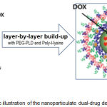Figure 1: Schematic illustration of the nanoparticulate dual-drug delivery system. Click here to View figure

 

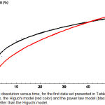Figure 2: Drug dissolution versus time, for the first data set presented in Table 1. Shown are the data points, the Higuchi model (red color) and the power law model (black color) which fits the data better than the Higuchi model.   Click here to View figure

 

Results and Dicussion

Model Comparison

We now proceed to perform the model comparison using the χ² minimization method. For a given data set with N number of time points with values Q_i and errors σ_i, i taking values from one to N, and for a given function f(t;a₁,a₂,…,a_m) that models the amount of drug as a function of time and is characterized by m free parameters (where N > m), we compute χ² using the standard formula:

where we sum over all experimental time points from i=1 to i=N, and thus χ² is a function of the free parameters that characterize the mathematical model. Minimizing χ² we determine the values of the parameters for which the model best fits the data, and finally we compute χ_min²/d.o.f, where d.o.f stands for the number of degrees of freedom given by N −m.

This last step is necessary in order to compare models with different number of free parameters.

In our analysis the models are characterized either by one or by two free parameters, and so m = 1 or m = 2, while the data sets have either 8, 10 or 12 points and so N = 8, N = 10 or N = 12.

For a given data set the model that best fits the data is the one with the lowest χ²_min /d.o.f. We start with the first data set seen in Table 1 and we minimize χ² for all models one by one using the computer software Mathematica.¹¹ By comparing χ²_min/d.o.f we see that the power law model has the best fit. The values of the parameters are summarized in Table 6, while as was illustrated in Figure 2, we can see that indeed the power law model fits the data way better than the Higuchi model.

Table 6: Values of parameters for first data set (N=10)

Model	First parameter	Second parameter	χ^2min/d.o.f
Higuchi (m = 1)	k = 10.6865h^(−1/2)	–	13.1467
Power law (m = 2)	A = 23.3605h^(−n)	n = 0.2856	1.4183
Hopfenberg (m = 1)	k = 1.5740h^(−1)	–	69.1869
Zero order (m = 2)	A = 35.7739	B = 0.7355h^(−1)	5.9920
Hixson-Crowell (m = 2)	A = 3.3535	B = 0.0164h^(−1)	7.0212
First order (m = 2)	Q0 = 38.4977	k = 0.0293h^(−1)	7.4994

 

We then follow exactly the same procedure for the rest of the data sets seen in Tables 2, 3, 4 and 5. Our results show that the power law model has the best fit in all cases, and therefore our conclusion is robust.

Our results are interesting for three reasons: Foremost, we have shown that although the most-widely used model in the literature is the one introduced by Higuchi,⁴ at least the class of systems considered here are best described by the power law model. In addition, we have shown that it is possible that a model with more parameters has a better fit to the data contrary to what is stated in the literature when the coefficient of determination R² is used.² This is due to the fact that although the number of degrees of freedom decreases when the number of free parameters increases, in some cases the χ² at the minimum is reduced so much that overall the χ²/d.o.f is lower. Finally, knowing the model that best describes the systems studied here in, it would be interesting to try to understand the underlying mechanism starting from basic principles, and relate the parameters of the model with properties of the system. In that case, since the parameters of the model have been already determined upon comparison with the data, one can compute the properties of the system, and thus the properties of the system could be measured experimentally using our method. Furthermore, it is interesting to note at this point that the power law time dependence can be mathematically derived as the exact analytical solution of the diffusion equation in one dimension in the semi-infinite domain x > 0:

C(t,x)_t = D C(t,x)_xx                                                                                                        (8)

where the sub index t denotes differentiation with respect to time, while the sub index xx denotes double differentiation with respect to space, with the initial condition C(t = 0,x) = 0  and boundary condition C(t,x = 0) = kt^n/2. In the above initial/boundary problem D is the diffusion coefficient assumed to be a constant, C(t,x) is the drug concentration as a function of time and position and k,n are constants. It is known from mathematical physics that this boundary/initial value problem is well posed and it has a unique solution.¹¹ Using the method of Laplace transform (see e.g.[11]) one finds that the unique solution that satisfies the diffusion equation and all conditions is the following¹²:

C(t,x) = kΓ(1 + n/2)(4t)^n/2 iⁿ erfc(x/2√Dt)                                            (9)

where Γ(z) is the Euler’s Gamma function, and we make use of the error function erf(x) and the complementary error function erfc(x) defined as follows:

erfc(x)=1−erf(x)                                                                                  (11)

For more details on the special functions of mathematical physics see e.g.¹³ Finally, given the drug concentration, we can now compute the amount of the drug as a function of time by performing the integral over all space from zero to infinity:

The integral can be computed exactly and finally we obtain:

M(t) =(k√DΓ(1 + n/2))/(2ⁿ Γ (3/2 + n/2)) t^(n+1/ 2)                             (13)

Conclusions

In this work, we conducted comparisons between several mathematical models widely-mentioned in the literature regarding predicting overall release behavior. We have used 5 different data sets obtained experimentally in realistic systems with different drugs and nanoparticles. Each model is characterized by one or two free parameters to be determined upon comparison with the data. We have used the χ² minimization method to determine the values of the parameters of each model, and we have obtained the minimum value of χ² per degree of freedom for each model. Our results show that among all mathematical models studied herein, the power law model has the best-fit in all 4 cases. We conclude that at least the class of systems considered here are best described by the power law model, characterized by two free parameters, although the Higuchi model is the most widely-used in the literature, and also despite other claims that adopting the coefficient of determination R², models with more parameters have a worse fit to the data. Finally, our derived method could in principle be used to measure variable properties of the nano-systems, experimentally.

Acknowledgments

BioMAT’X Research Group, part of CIIB (Centro de Investigación e Innovación Biomédica), Faculty of Dentistry, Universidad de los Andes, Santiago de Chile. 

Funding

The corresponding author acknowledges supplementary operating funding provided from CONICYT-FONDEF Chile under awarded project/grant (national) # ID16I10366 (2016-2019) and Fondo de Ayuda a la Investigacion FAI – Universidad de los Andes No. INV-IN-2015-101 (2015-2019). 

Conflicts Of Interest

None.

References

1.  Shaikh K. H.,  Kshirsagar R. V., Patil S. G. Mathematical Models for Drug Release Characterization: A Review. World Journal of Pharmacy and Pharmaceutical Sciences. 4(4).
2.  Lokhandwala H., Deshpande A and Despande S. Kinetic Modeling and Dissolution Profiles Comparison: An overview. Int J Pharm Bio Sci. 2013;4(1):728 737.
3.  Dash S.,Murthy N. P., Nath L.,  Chowdhury P. Kinetic Modeling on Drug Release from Controlled Drug Delivery Systems. Acta poloniae pharmaceutica. 2010;67(3):217-23.
4. Higuchi T. Mechanism of sustained-action medication theoretical analysis of rate of release of solid drug dispersed in solid matrices. J. Pharm. Sci. 1963;52:11451149.
   CrossRef
5. Hixson  A. W.,Crowell  J. H. Dependence of reaction velocity upon surface and agitation I theoretical consideration. Ind. Eng. Chem. 1931;23:923931.
   CrossRef
6. Korsmeyer R. W.,Gurny R., Doelker E., Buri  P., Peppas N. A. Mechanisms of solute release from porous hydrophilic polymers. Int J Pharm. 1983;15:2535.
   CrossRef
7. Hopfenberg H. B., In: Paul  D. R., Harris F. W. (Eds.), Controlled Release Polymeric Formulations. ACS Symposium Series 33. American Chemical Society, Washington, DC. 1976;2631
8.  Ramasamy T., Haidar S. Z., Tran H. T.,Choi Y. J., Jee-Heon J., Shin S. B., Han-Gon C., Yong S. C.,   Kim O. J. Layer-by-Layer Assembly of Liposomal Nanoparticles with PEGylated Polyelectrolytes Enhances Systemic Delivery of Multiple Anticancer Drugs. Acta Biomaterialia.  2014;10(12).
   CrossRef
9. Wu Y.,  Wang Z.,  Liu G., Zeng X., Wang X., Gao Y., Jiang L.,  Shi X., Tao W., Huang L and  Mei L. Novel Simvastatin-Loaded Nanoparticles Based on Cholic Acid-Core Star-Shaped PLGA for Breast Cancer Treatment. Journal of Biomedical Nanotechnology.  2015;11:12471260.
   CrossRef
10. Katzer T., Chaves P., Bernardi A., Pohlmann A., Guterres S. S., Beck R. C. R. Prednisolone loaded nanocapsules as ocular drug delivery system: developement, in vitro drug release and eye toxicity. J. Microencapsul. 2014;31(6):519-28.
    CrossRef
11. http://www.wolfram.com/
12.   Arfken B. G., Weber J. H. Mathematical Methods for Physicists, Elsevier Academic Press, sixth edition.
13. Crank J.  The Mathematics of Diffusion, Brunel University Uxbridge, second edition.

(Visited 1,087 times, 1 visits today)