Sumit Kushwaha

Electronics Engineering Department, Kamla Nehru Institute of Technology, Sultanpur, India.

Corresponding Author E-mail: sumit.kushwaha1@gmail.com

DOI : https://dx.doi.org/10.13005/bpj/1240

Abstract

Ultrasound (US) imaging is a valuable imaging technique for clinical diagnosis. It is non-invasive in nature and imaging the internal structure of the body to identify the probabilistic diseases or, abnormalities in tissues behavior. However, inherent response of speckle noise in US images limit the fine and edge details which affect the contrast resolution. This makes clinical diagnosis more difficult.In this paper, we proposed a non-linear anisotropic diffusion filtering for speckle reduction approach based on non-linear progression partial differential equation (PDE). For analysis purpose, we have considered the set of eight-real clinical B-Mode US images of human liver from different patient. These real US images are used for quantitative analysis. We compare the performance of four speckle reduction filters as Perona-Malik Filter, LEE Filter, FROST Filter, ADMBSS Filter with our proposed filter in terms of peak signal to noise ratio (PSNR) value performance index under various noise variance selection Parmenter. Finally, we see that our proposed approach preserves the clinical details in US images and minimizing the noise level. Results for set of eight US images shows that our proposed filtering approach is more efficient for speckle noise reduction in comparison to other discussed filters in term of higher PSNR value (dB).

Keywords

Diffusion filter; MATLAB;PDE; PSNR;Ultrasound;

Download this article as: 

Copy the following to cite this article: Kushwaha S. An Efficient Filtering Approach for Speckle Reduction in Ultrasound Images. Biomed Pharmacol J 2017;10(3).

Copy the following to cite this URL: Kushwaha S. An Efficient Filtering Approach for Speckle Reduction in Ultrasound Images. Biomed Pharmacol J 2017;10(3). Available from: http://biomedpharmajournal.org/?p=16002

Introduction

Medical Ultrasound (US) Imaging technique is a non-ionizing radiations imaging modality that enables real time diagnosis treatment. This technique has non-invasive nature. It is widely used in medical field for diagnosis, patient routine check-ups for good health, and more and more use in surgeries and intrusions as a supervision modality. This inferior image quality is a challenging issue in US imaging as compared to other imaging modalities. The degree of degradation in US image quality can be highly varying and it depends on patients to patients. Sometimes it is an important challenge to imaging desired structures in particular pose of a fatty patient.^1,2 US images suffers from numerous acoustic imaging objects including resonance, deviations and effect of speckle noise. In this paper, we focused on minimization of speckle noise effect in US images. Speckle noise effect seems like a granular texture effect on the US image. It is an inherent response of the backscattered interfering signal from the desired interrogated medium.³ In fact, an accurate description of the speckle noise pattern statistics is still an active research area which involves complex analytical modelling. Speckle noise behavior statistics may be characterized into different modules.⁴ Speckle noise effect is spatially correlated with correlation length which is calculated by the autocorrelation of the point spread function (PSF). In various US imaging cases, need for depth of diffusion leads to important speckle correlation lengths.

Earlier speckle reduction LEE filter⁵ and FROST filter⁶ were believed that speckle noise has additive and multiplication noise component in it. These filters are suitable for speckle reduction by minimizing mean squared error (MSE). These filter statistics are based estimation in local windows. The limitations with these filters are that it smoothed the image near structured and edges region. Perona and Malik filter⁷ is firstly adopted the anisotropic diffusion technique for speckle noise reduction in US Images. This filter avoids the unnecessary smoothing related with linear diffusion techniques, but not preserve edges details. A recent speckle reduction method ADMBSS filter⁸ proposes a memory based on speckle statistics filtering. This simple technique aims to apply memory mechanism as delay differential equation (DDE) for the diffusion tensor. The behavior of this memory mechanism follows the statistics of the tissues and preserves the clinical details in US images.

Finally, the main challenges with US filtering techniques are preserving the relevant clinical details and avoiding over filtering problem. Keep in mind these limitations and challenges of state-of-the-art filters, we proposed an efficient anisotropic diffusion filter for speckle reduction in US images. Our proposed filter gives better result for experiment with eight real US test images of different patients. This is the novelty of our proposed work.

Related Studies

Lee Filter For Speckle

The Lee filter reduces the speckle noise by applying a spatial filter to each pixel in an image, which filters the data based on local statistics calculated within a square window. The value of the center pixel is replaced by a value calculated using the neighboring pixels.^4,5 This pointwise linear filter is based on the Minimum Mean Square Error (MMSE), and produced speckle noise free image based on the following equation (value of filtered pixel):

where,

and

and

K= weight function,

P_c—Center pixel value of kernel/window (Median value)

L_m—Local mean of filter window

L_v—Local variance of filter window

M—Multiplicative noise mean (Default value: 1)

MV—Multiplicative noise variance (Default value: 0.25)

N Looks—Number of looks (Specifies the number of looks of the image. This is used to calculate the Multiplicative noise variance and control the amount of smoothing applied to the image. Using a smaller value for the Number of Looks leads to more smoothing, and a larger value preserves more image features.⁹)

The N Looks for a homogeneous region of an image is the ratio between the mean squared to the variance. The Looks is defined as follows:

The local mean L_m of filter window is defined as:

Similarly, the local variance L_v of the filter window is defined as:

From eq. (4), if value of L_v is negative, in that case we have a very homogeneous area, L_v should be set to zero. Then estimate

is given by the local mean L_m If value of L_v is very high, this indicates a very high contrast region (or, an edge presence) and

=f (x, y, z). These extreme cases are in accordance with the Bayesian approach that is adopted in this linear MMSE filter.5

Frost Filter For Speckle

The FROST filter is used to design an adaptive filter algorithm to reduce speckle noise in spatial domain and computationally very efficient. This filter preserves the important features of image at the edges. It is a MMSE convolutional filter for speckle reduction. The Frost filter is an exponentially damped circularly symmetric filter that uses local statistics within individual filter windows. The pixel being filtered is replaced with a value calculated based on the distance from the filter center, the damping factor, and the local variance. The Frost filter requires a damping factor (define the extent of smoothing). The Damping Factor value defines the extent of exponential damping. The smaller the value is, the better the smoothing ability and filter performance. After application of the Frost filter, the denoised images show better sharpness at the edges.^6,10,11 The algorithm used in the implementation of the Frost filter is as follows:

From eq. (1):

where,

K = e^-(B*S),

where,

and

S—Absolute value of the pixel distance from the center pixel to its neighbors in the filter window,

D—Exponential damping factor (Default value:1)

The factor D is chosen such that when in a homogeneous region, B approaches zero, yielding the mean filter output; at an edge B becomes so large that filtering is inhibited completely.¹²

Perona Malik Filter

Perona Malik filter is a classical diffusion filter technique for speckle reduction in US images. This diffusion filter is a linear and space invariant transformation of the original image. The resulting image in this filter obtained by convolution between the images and an isotropic Gaussian filter.¹³ Perona and Malik⁷ have given a name to their filter called anisotropic diffusion filter. This diffusion filter technique typically looks like the process that creates a scale space not a diffusion tensor, where an image generates a parameterized family of successively more and more blurred images based on a diffusion process.Diffusion is a physical process to create equilibrium concentration differences without destroying or, creating body mass. The Perona Malik filter is based on the equation:

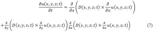
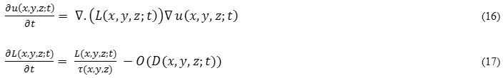
with initial condition u_o (x, y, z) = u (x, y,z: t =0) which is noisy image/input image. u (x, y, z: t) is the output image. D (x, y, z: t) is diffusion coefficient, known as symmetric positive definite tensor. D (x, y, z: t) also controls the rate of the diffusion. D (x, y, z: t) depends on local structure of  u (x, y,z: t) (if D is constant, then filter is isotropic diffusion filter and if D is not constant, then filter is anisotropic diffusion filter) and ∇. and  ∇ denote the divergence operator and gradient operator, respectively, u_o (x, y, z)  is the initial image, i.e. noisy image, t is temporal variable. Eq. (7), Linear Anisotropic Diffusion (LAD), is an elliptic Partial Differential Equation (PDE).¹⁴

By using finite difference method, eq. (7) given as:

which is expressed as

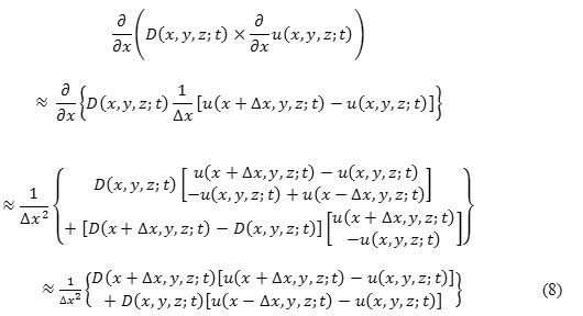
where “≈” shows that the R.H.S. part of the equation is the difference approximation of the L.H.S. part.

Similarly, we have

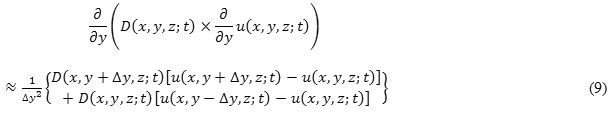
and,

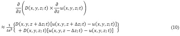
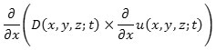
All the values of eq. (8), eq. (9), and eq. (10) inserting in eq. (7) to obtain difference approximation of

Pu Δx = 1, Δy = 1, and Δz = 1we get:

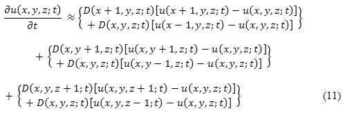
So, obtaining discrete realization of anisotropic diffusion filter for u (x, y,z: t) image from eq. (11):

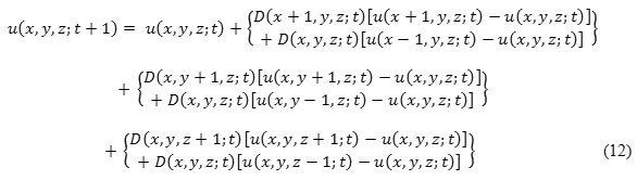
In eq. (12), we can see that the major problem is selection of diffusion coefficient D (x, y,z: t) in anisotropic diffusion filter.

Diffusion coefficient D (x, y,z: t) is calculated as¹⁵:

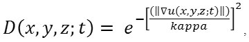
when diffusion occurs across the boundaries and applies it in homogeneous areas. and,

When diffusion occurs near the boundaries and applies it in homogeneous areas.

Where, kappa is the gradient modulus threshold that controls the diffusion coefficient. Also, kappa controls the sensitivity near the edges and chosen experimentally or as a function of the noise in the image (kappa > 0).

Anisotropic Diffusion for Memory Based on Speckle Statistics (ADMBSS) Filter

ADMBSS filter⁸is to eliminate the effect of gradient information due to the lack of contours and low contrast of US images with objective of preservation of relevant clinical details in interest region using probabilistic-driven selective memory mechanism filtering. This filter is adapted to the US medical imaging context.⁹ For preserving clinical information in US images, G. Ramos-Llordénet. al.⁸ consider two different methods for tissue classification. 1^st selective diffusion tensor method and 2^nd probability driven memory methods in region of interest for tissue classification

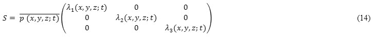
A selective filtering tensor operator 0 (x, y, z: t) used as transformation of the instantaneous diffusion tensor D (x, y, z: t) at location (x, y, z) into a null tensor for suitable tissue classification and preservation. In this context, p (x, y, z: t) = 1 – p (x, y,z: t) for the probability of the tissue regions and p (x, y, z: t) for the probability of the non-tissue (meaningless) regions. For this selective behavior, the diffusion tensor D (x, y, z: t) is multiplied by its Eigenvalues by  p (x, y, z: t). Memory mechanism used, to know the anisotropic diffusion direction satisfy the condition that  p (x, y, z: t) → 0, so τ (x, y, z)  p (x, y, z: t) → ∞ . Memory mechanism will be disable if  p (x, y, z: t) → 1, so that τ (x, y, z)  p (x, y, z: t) → 0.  So the new reconstruct diffusion tensor by using expansion of outer product:

where

and,

Preserving pathway of the time dependent probability for getting more robust characterization than obtained from instantaneous probability, p (x, y, z: t),  tensor operator O (x, y, z: t) is not directly applied to  L (x, y, z: t). This p (x, y, z: t) provides more robust characterization than p (x, y, z: t).

Now, delay differential equation (DDE), with same initial and periodic condition as [10] and τ (x, y, z) is the spatial dependence of  τ, will be:

Where, L (x, y, z: t) is the diffusion tensor matrix at point (x, y, z) and time t. Integrate eq. (52), we get:

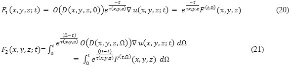
To turn ON/OFF the memory mechanism, spatial dependence τ (x, y, z) should satisfied the minimum conditions that τ (x, y, z): [0,1] → (0, ∞). The anisotropic diffusion flux  F (x, y, z: t) = L (x, y, z: t) ∇ u (x, y, z: t), then from eq. (18):

Where filtered diffusion tensor

and

Proposed Non-Linear Anisotropic Diffusion Filter

Most of the diffusion filters are simply modifications of perona-malik filter [7] where D is constant (scalar coefficient based on gradient of the image D ∇ u (x, y, z: t) which avoids diffusion near the boundaries and applies it in homogeneous areas). Here, we propose an efficient non-linear anisotropic diffusion for speckle reduction filtering approach based on non-linear progression of PDE. This proposed filter selects finite power intensity image u_o (x, y, z) and having none zero-valued intensities over the image domain Ω. Here,

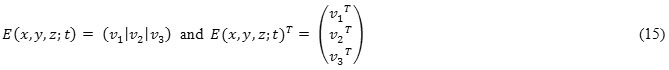
is a given field of symmetric positive definite diffusion tensors where Ω is an open region of ³ and ∂Ω is boundary of Ω. Eigenvectors  { v_{1 ,} v_{2 ,} v_3 ,} of these tensors define preferential diffusion directions, and the Eigenvalues their corresponding coefficients. Evolution rule eq. (6) is complemented with an initial condition u (x, y, z; 0) = u_o (x, y, z) at time t = 0. If  has pixels of vector type, then their components are treated independently.^5,16 We get the output image u (x, y, z; t) by following PDE:

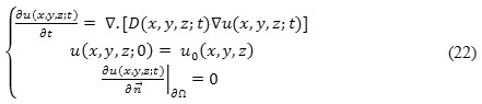
where ∂Ω denotes the boundary of

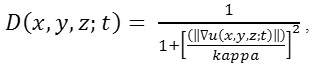
is the outer normal to the ∂Ω, and D (x, y, z)  is coefficient of diffusion which is defined as a decreasing function of the instantaneous coefficient of variation.

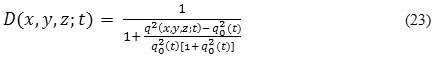
or,

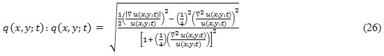
In eq. (23) and (24), q (x, y, z; t) is the instantaneous coefficient of variation serves as the edge detector in speckled imagery, q_o (t) is the speckle scale function and is estimation parameter related to the coefficient of variation of noise. q (x, y, z; t) is determined by:

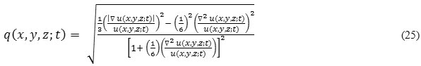
In case of 2-D, instantaneous coefficient of variation

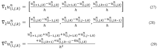
Here, four stage iterative method can be used to solve mathematically. Let anisotropic diffusion time step ∇ t  and spatial step h in x, y, z directions respectively, then the discretization of time and space coordinates as t = n Δ t; n = 0, 1, 2, 3, … … and x = ih, y = jh, z = kh; i = 0,1,2,3, … … ., M – 1, j =0,1,2,3, … , N – 1, k = 0,1,2,3, … … . , k – 1 respectively, where Mh x Nh x kh is support image size.For mathematical applications, we choose h = 1, and Δ t = 0.05. Let

then iterative method can be described as:

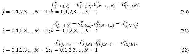
Here, we are using symmetric boundary conditions. So:

Experiment and Discussion

In this experiment, we have considered the set of eight-real clinical B-Mode US images of human liver from different patient.^17,18 These real US images are used for quantitative analysis. The size of these real clinical B-Mode US images of human liver is 256 x 256 x 24 (in pixel unit) in x, y, and z directions respectively. This data set is fed into the MATLAB¹⁹ platform for quantitative analysis. For measuring the all filters performance, we have used Peak Signal to Noise Ratio (PSNR) value (measured in dB).²⁰ Higher PSNR value means higher level of image quality reconstruction. We have tested the performance of the filters (LEE Filter,⁵ FROST Filter,⁶ Perona Malik Filter,⁷ ADMBSS Filter⁸ and Proposed Filter) for all US images under different noise variance as 0.01, 0.04, 0.07, 0.1, and 0.5. All quantitative analysis results are represented in table form from Table I to VIII, and also shown in graphical form in figure 2. The output image of all filters under different noise variances are shown sequentially from figure 3 to figure 7. Now, we have seen that our proposed filter gives higher PSNR value under different noise variances in comparison to other discussed filters. This shows that our proposed filter is work efficiently for speckle noise reduction in US images under different noise variances.

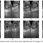Figure 1: Experiment results obtain from these eight B-mode US images of human liver.   Click here to View figure

 

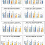Figure 2: The graphs are plotted for PSNR result values for different filters. These graphs show that our proposed filter is more efficient for removing Speckle noise.   Click here to View figure

 

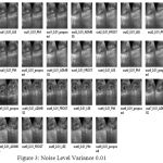Figure 3: Noise Level Variance 0.01   Click here to View figure

 

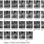Figure 4: Noise Level Variance 0.04   Click here to View figure

 

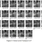Figure 5: Noise Level Variance 0.07   Click here to View figure

 

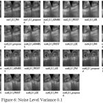Figure 6: Noise Level Variance 0.1   Click here to View figure

 

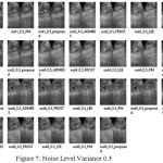Figure 7: Noise Level Variance 0.5   Click here to View figure

 

Table 1: Performance Comparison of Different Filters for Image 1

PSNR(dB) RESULTS FOR THE IMAGE 1 EXPERIMENT
Noise Level	Perona Malik Filter	LEE Filter	FROST Filter	ADMBSS Filter	Proposed Filter
0.01	33.5863	30.7646	27.9208	33.0753	59.9532
0.04	26.8198	25.5545	24.1795	33.8953	52.0865
0.07	24.2403	23.0597	22.0432	43.5523	43.3213
0.1	22.8419	21.5929	20.7415	37.116	39.3994
0.5	18.6482	15.4397	15.0582	34.3762	28.4605

Table 2: Performance Comparison of Different Filters for Image 2

PSNR(dB) RESULTS FOR THE IMAGE 2 EXPERIMENT
Noise Level	Perona Malik Filter	LEE Filter	FROST Filter	ADMBSS Filter	Proposed Filter
0.01	31.8765	29.6114	27.4193	38.7373	60.1176
0.04	25.3038	24.1023	23.0549	37.0798	46.9497
0.07	23.1179	21.8245	21.0142	54.1903	39.5293
0.1	21.8242	20.3137	19.6463	47.3763	36.3813
0.5	18.2999	14.5549	14.2363	42.1617	27.4346

Table 3: Performance Comparison of Different Filters for Image 3

PSNR(dB) RESULTS FOR THE IMAGE 3 EXPERIMENT
Noise Level	Perona Malik Filter	LEE Filter	FROST Filter	ADMBSS Filter	Proposed Filter
0.01	33.6423	30.7505	27.9583	31.5686	60.4925
0.04	26.838	25.6038	24.1918	31.7607	51.1155
0.07	24.3578	23.1577	22.1389	44.7001	43.5445
0.1	22.8507	21.5427	20.7171	29.142	38.5877
0.5	18.6508	15.4617	15.0717	39.746	28.6693

Table 4: Performance Comparison of Different Filters for Image 4

PSNR(dB) RESULTS FOR THE IMAGE 4 EXPERIMENT
Noise Level	Perona Malik Filter	LEE Filter	FROST Filter	ADMBSS Filter	Proposed Filter
0.01	31.8291	29.5409	27.3701	37.9569	61.7416
0.04	25.2852	24.0751	23.0358	34.5986	45.9795
0.07	23.1725	21.8448	21.0474	50.9217	39.4964
0.1	21.8462	20.3749	19.6957	41.2622	36.0276
0.5	18.2611	14.545	14.2376	43.3388	27.3917

Table 5: Performance Comparison of Different Filters for Image 5

PSNR(dB) RESULTS FOR THE IMAGE 5 EXPERIMENT
Noise Level	Perona Malik Filter	LEE Filter	FROST Filter	ADMBSS Filter	Proposed Filter
0.01	32.7224	29.9306	27.1693	45.0071	59.175
0.04	27.2024	25.7441	24.1846	41.735	52.7133
0.07	24.9565	23.6137	22.4323	38.3478	44.5785
0.1	23.5763	22.1666	21.1989	40.7795	40.0525
0.5	19.3568	16.1321	15.705	42.24	29.3316

Table 6: Performance Comparison of Different Filters for Image 6

PSNR(dB) RESULTS FOR THE IMAGE 6 EXPERIMENT
Noise Level	Perona Malik Filter	LEE Filter	FROST Filter	ADMBSS Filter	Proposed Filter
0.01	34.1398	31.1547	28.1883	32.4728	60.5218
0.04	25.2852	26.0935	24.6419	28.4759	53.269
0.07	24.9829	23.8935	22.6956	33.6521	44.4787
0.1	23.474	22.2108	21.3055	32.4591	40.083
0.5	18.9455	15.9552	15.5656	43.2921	29.074

Table 7: Performance Comparison of Different Filters for Image 7

PSNR(dB) RESULTS FOR THE IMAGE 7 EXPERIMENT
Noise Level	Perona Malik Filter	LEE Filter	FROST Filter	ADMBSS Filter	Proposed Filter
0.01	33.7113	30.9191	28.3638	36.439	60.8786
0.04	27.2024	25.6571	24.4113	44.4852	49.149
0.07	24.6137	23.355	22.4096	34.3248	41.7057
0.1	23.2736	21.9426	21.1419	29.9298	38.9144
0.5	19.0164	15.8372	15.4541	18.3136	29.0295

Table 8: Performance Comparison of Different Filters for Image 8

PSNR(dB) RESULTS FOR THE IMAGE 8 EXPERIMENT
Noise Level	Perona Malik Filter	LEE Filter	FROST Filter	ADMBSS Filter	Proposed Filter
0.01	31.4013	28.6532	26.1152	38.0811	62.3628
0.04	25.9988	24.4407	23.009	39.4908	49.7713
0.07	24.7752	22.3701	21.2703	40.2364	41.8029
0.1	22.447	20.9436	20.0514	26.1845	38.1168
0.5	18.6631	15.1269	14.7353	20.7533	28.1388

Conclusion

Speckle noise is inherent response in US images. Since it degraded the image quality and affecting fine and edge details. So, it is difficult task to see the clinical details in patient diagnosis. In this paper, we proposed a non-linear anisotropic diffusion filtering based speckle reduction approach based on non-linear progression PDE. This approach minimizes the speckle noise, preserves the clinical diagnosis details of patient. The experimental analysis tested on set of eight-real clinical B-Mode US images of human liver from different patientunder various noise variance selection Parmenter. We compare the performance of Perona-Malik Filter, LEE Filter, FROST Filter, ADMBSS Filter with our proposed non-linear anisotropic diffusion based speckle reduction filter.  We see that our proposed approach preserves the clinical details in US images and minimizing the noise level in term of higher PSNR value (dB). This is very helpful approach for radiologists/Doctors to accurate clinical diagnosis. Future works will include speckle reduction for more real time US images as well as in real time US imaging video.

References

1.  Destrempes F and  Cloutier G. A critical review and uniformized representation of statistical distributions modeling the ultrasound echo envelope.Ultrasound Med. Biol. 2010;36(7):1037–51.
   CrossRef
2. Tay P. C.,  Garson C. D., Acton S. T and Hossack J. a. Ultrasound despeckling for contrast enhancement. IEEE Trans. Image Process. 2010;19(7):1847–60.
   CrossRef
3. Rabbani H., Vafadust M.,  Abolmaesumi P and  Gazor S. Speckle noise reduction of medical ultrasound images in complex wavelet domain using mixture priors. IEEE Trans. Biomed. Eng. 2008;55(9):2152–60.
   CrossRef
4. Krissian K.,  Westin C. F.,Kikinis R and Vosburgh K. G. Oriented speckle reducing anisotropic diffusion. IEEE Trans. Image Process. 2007;16(5):1412–1424.
   CrossRef
5. Jean-Marie M., Jer^ome F., Risser L andTobji S. Anisotropic Diffusion in ITK.  arXiv: 1503.00992v1 [cs.CV]. 2015.
6.  Frost V.,Stiles J.,  Shanmugan K and Holzman J. A model for radar images and its application to adaptive digital filtering of multiplicative noise. IEEE Trans. PAMI. 1982;4(2):157–166.
   CrossRef
7. Perona P and Malik J. Scale-space and edge detection using anisotropic diffusion. IEEE Trans. Pattern Anal. Mach. Intell. 1990;12(7):629–639.
   CrossRef
8.  Ramos-Llordén G., Vegas-Sánchez-Ferrero G., Martin-Fernandez M., Alberola-López C and Aja-Fernández S. Anisotropic Diffusion Filter With Memory Based on Speckle Statistics for Ultrasound Images. in IEEE Transactions on Image Processing. 2015;24(1):345-358.
   CrossRef
9.  Cottet G. H and Ayyadi M. E. A Volterra type model for image processing. IEEE Trans. Image Process. 1998;7(3):292–303.
   CrossRef
10. Krissian K., Westin C. F., Kikinis R and Vosburgh K. G. Oriented speckle reducing anisotropic diffusion. IEEE Trans. Image Process. 2007;16(5):1412–1424.
    CrossRef
11.  Yu Y and  Acton S. T. Speckle reducing anisotropic diffusion. IEEE Trans. Image Process. 2002;11(11):1260–1270.
    CrossRef
12. Yu Y and Acton S. Edge detection in ultrasound imagery using the instantaneous coefficient of variation. IEEE Transactions on Image Processing. 2004;13(12):1640–1655.
    CrossRef
13.  Weickert J.  Anisotropic Diffusion in Image Processing, Stuttgart, Germany: Teubner. 1998.
14. Krissian K.,  Westin C. F.,Kikinis R and Vosburgh K. G. Oriented speckle reducing anisotropic diffusion. IEEE Trans. Image Process. 2007;16(5):1412–1424.
    CrossRef
15.  Aja-Fernandez S and Alberola-Lopez C. On the estimation of the coefficient of variation for anisotropic diffusion speckle filtering. IEEE Transactions on Image Processing in press.  2005;15(9):2694– 2701.
    CrossRef
16.  Cottet G. H and Ayyadi M. E. A Volterra type model for image processing. IEEE Trans. Image Process.  1998;7(3):292–303.
    CrossRef
17. Ultrasound Images Ultrasound images of diseases of the liver Accessed on 21st December. 2016. Available at http://www.ultrasound-images.com/liver/.
18. Online Medical Images, Ultrasound Images, Accessed on 21st December. 2016, Available at http://www.onlinemedicalimages.com/index.php/en/site-map.
19. MATLAB – Mathworks. The Language of Technical Computing tool, version R 2016, website: https://www.mathworks.com. 
20. Peak Signal-to-Noise Ratio (PSNR) – MATLAB psnr – MathWorks India, available online at: http://in.mathworks.com/help/images/ref/psnr.html.

(Visited 1,386 times, 1 visits today)