R. Murugan¹, Reeba Korah², T. Kavitha³

 ¹Research Scholar, Centre for Research, Anna University, Chennai, 600025, India ²Professor, Alliance College of Engineering and Design, Alliance University, Bangaluru, 562106, India ³Professor, Valliammai Engineering College, Chennai, 603203, India *Corresponding author E-mail: murugan.rmn@gmail.com  

DOI : https://dx.doi.org/10.13005/bpj/630

Abstract

Optic disc detection is an important step in retinal image screening process. This paper proposes an Automatic detection of an optic disc in retinal fundus images. The manual method graded by clinicians is a time consuming and resource-intensive process. Automatic retinal image analysis provides an immediate detection and characterization of retinal features prior to specialist inspection. This proposed a binary orientation technique to detect optic disc, which provides higher percentage of detection than the already existing methods. The method starts with converting the RGB image input into its LAB component. This image is smoothed using bilateral smoothing filter. Further, filtering is carried out using line operator. After which gray orientation and binary map orientation is carried out and then with the use of the resulting maximum image variation the area of the presence of the OD is found. The portions other than OD are blurred using 2D circular convolution. On applying mathematical steps like peak classification, concentric circles design and image difference calculation, OD is detected. The proposed method was implemented in MATLAB and tested by publically available retinal datasets such as STARE, DRIVE. The success percentage was found to be 98.34% and the comparison is done based on success percentage.  

Keywords

Optic disc; diabetic retinopathy; mathematical morphology; template matching; optimization; binary orientation

Download this article as: 

Copy the following to cite this article: Murugan R, Korah R, Kavitha T. Computer Aided Screening of Optic Disc in Retinal Images Using Binary Orientation Map. Biomed Pharmacol J 2015;8(1)

Copy the following to cite this URL: Murugan R, Korah R, Kavitha T. Computer Aided Screening of Optic Disc in Retinal Images Using Binary Orientation Map. Biomed Pharmacol J 2015;8(1). Available from: http://biomedpharmajournal.org/?p=2124>

Introduction

The detection of optic disc (OD) is a first step for the diagnosis of different pathologies of retinal diseases such as glaucoma, diabetic retinopathy. The optic disc is in a vertical oval shape with the horizontal and vertical average dimension of 1.76mm and 1.92mm respectively. It is located  at  the  distance  of  3  to  4mm  from  the  nasal  side  of fovea (Haseeb  Ahsan, 2015)¹.The  dimension  of  optic  disc  varies  from  person  to person but its diameter remains the  same (80-100 pixels) for standard fundus  image (Peter H. Scanlon,2015)².The optic disc is a bright yellowish disc  that  transmits  electrical  impulses  from  retina  to  brain where  the  occurrence  of  blood  vessels and  optic  nerve  fibre  takes place (David et al., 2015)³ .The optic disc does not contain any receptors hence it is also called as blind spot. The OD vicinity consists of large vessels that are used for vessel tracking methods. For any  retinal  fundus  image  OD  occupies  about  one  seventh  of the entire image.  The health status of the human retina can be determined from the physical characteristics of OD (Ahmed et al., 2015)⁴.

There are many approaches ^(5-19) that have been proposed for the automatic detection of OD.  The proposed OD detection methods are categorized as mathematical morphology ^(5-9), segmentation algorithms ^(10-15), Optimization^(16-18) and template matching⁽¹⁹⁾. Mathematical morphology plays a major role in retinal image

 

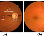Figure 1: (a) Retinal image landmarks (b) OD localized  image Click here to view full figure

 

processing that includes dilation, erosion, opening and closing. The different techniques that are implemented in mathematical morphology for the detection of optic disc are Principle  Component  Analysis (PCA) (Sinthanayothin et al.,2010)⁵,  morphological based  edge  detection (Arturo  Aquino et al., 2010)⁶,  vessel  direction  matched  filter  method (Aliaa  Abdel et al.,2008)⁷, Sobel  operator (Abdel-Ghafar  et al.,2007)⁸ and bit  plane  slicing(Ashok  kumar et al 2012)⁹.

Segmentation algorithms uses to divides the fundus image into multiple segments in order to locate OD and its boundaries. This methods are vessel  classification (Jeline 2010)¹⁰,   thresholding (F.  ter  Haar ,2005)¹¹,  Snake method(Alireza  Osareh  et al., 2002)¹², Active contour(Gopal  Datt  Joshi et al.,2010)¹³, Deformation  contour  method  (Juan  Xu et al.,2006)¹⁴ and Wavelet transform(Pallawala et al.,2004)¹⁵. Optimization  technique  are used to locate OD, these methods includes fuzzy  convergence(Kenneth et al.,2006)¹⁶,  Forward  selection   and  backward elimination(Bowd et al.,2002)¹⁷ and KNN regressor (Niemeijer  et al.,2009)¹⁸.The template based methods are also used to localize OD these method hausdorff template matching(Marc  Lalonde  et al.,2001)¹⁹.

Material

Two publicly available datasets were used to test the proposed method. The STARE subset ⁽²⁰⁾ contains 81 fundus images that were used for evaluating their automatic OD localization method. The images were captured using a Top Con TRV-50 fundus camera at 35o field-of-view (FOV), and subsequently digitized at 605 X 700, 24-bits pixel. The dataset contains 31 images of normal retinas and 50 of diseased retinas.

The second dataset used is the DRIVE dataset ⁽²¹⁾, established to facilitate comparative studies on retinal OD localization. The dataset consists of a total of 40 color fundus photographs used for making actual clinical diagnoses, where 33 photographs do not show any sign of diabetic retinopathy and seven show signs of mild early diabetic retinopathy. The –24 bits, 768 by 584 pixels color images are in compressed JPEG-format, and acquired using a Canon CR5 non-mydriatic 3CCD camera with a 45^o FOV.

Methodology

This section presents the proposed OD detection technique. In particular, we divide this section into four subsections, which deal with the retinal image pre-processing, designed line operator, OD detection, and discussion, respectively.

Retinal Image Pre-processing

Retinal images need to be pre-processed before the OD detection. As the proposed technique makes use of the circular brightness structure of the OD, the lightness component of a retinal image is first extracted. We use the lightness component within the LAB color space, where the OD detection usually performs the best (Osareh et al.,2002). For the retinal image in Fig. 1(a), Fig. 2(a) shows the corresponding lightness image.The retinal image is then smoothed to enhance the circular brightness structure associated with the OD. We use a bilateral smoothing filter (Tomasi et al.,1998) that combines geometric closeness and photometric similarity as follows:

h(x) = k(x) c(ξ, x) s(f(ξ); f(x)) d ξ (1)

With the normalization factor

k(x) = s(f(ξ); f(x)) d ξ                            (2)

where f (x) denotes the retinal image under study. c(ξ, x) and s(f(ξ), f (x)) measure the geometric closeness and the photometric similarity between the neighborhood center x and a nearby point ξ. We set both c(ξ, x) and s(f(ξ), f(x)) by Gaussian functions. The geometric spread σd and the photometric spread σr of the two Gaussian functions are typically set at 10 and 1 as reported in [23]. For the retinal image in Fig. 2(a), Fig. 2(b) shows the filtered retinal image.

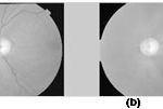Figure2: Retinal mage pre-processing. (a) Lightness of the example retinal image in LAB color space. (b) Enhanced retinal image by bilateral smoothing where multiple crosses along a circle label the pixels to be used to illustrate the image variation along multiple oriented line segments.   Click here to view full figure

 

Line operator

A line operator is designed to detect circular regions that have similar brightness structure as the OD. For each image pixel at (x, y), the line operator first determines n line segments L_i, i = 1. . . n of specific length p (i.e., number of pixels) at multiple specific orientations that center at   (x, y). The image intensity along all oriented line segments can thus be denoted by a matrix      I(x,y)nxp, where each matrix row stores the intensity of p image pixels along one specific line segment. The line operator that uses 20 oriented line segments and sets the line length   p = 21, each line segment Li at one specific orientation can be divided into two line segments L_i,1 and L_i,2 of the same length (p − 1)/2 by the image pixel under study (i.e., the black cell). The image variation along the oriented line segments can be estimated as follows:

D_i(x,y) =║ f_mdn (Il_i,1(x,y)) – f_mdn (Il_i,2(x,y)) ║, i=1…n         (3)

Where f_mdn (·) denotes a median function.  fmdn (Il_i,1 (x, y)) and fmdn (Il_i,2 (x, y)) return the median image intensity along L_i,1and L_i,2,respectively. D = [D_i(x, y)..D_i (x, y). . .D_n (x, y)] is, therefore, a vector of dimension n that stores the image variations along n-oriented line segments.

The orientation of the line segment with the maximum/minimum variation has specific pattern that can be used to locate the OD accurately. For retinal image pixels, which are far away from the OD, the orientation of the line segment with the maximum/minimum variation is usually arbitrary, but for those around the OD, the image variation along Lc [labeled in Fig. 1(b)] usually reach the maximum, whereas that along Lt reaches the minimum. Fig. 4 shows the image variation vectors D(x, y) of eight pixels that are labeled by crosses along a circle shown in Fig. 2(b). Suppose that there is a Cartesian coordinate system centered at the OD, as shown in Fig. 2(b). For the retinal image pixels in quadrants I and III, the image variations along the 1st–10th [i.e., L_t in Fig. 1(b)] and the 11th–20th (i.e., L_c ) line segments labeled in Fig. 3 reach the minimum and the maximum, respectively, as shown in Fig. 4. But for the retinal image pixels in quadrants II and IV, the image variations along the 1st–10th and the 11th–20th line segments instead reach the maximum and the minimum, respectively.

An orientation is constructed based on the orientation of the line segment with the maximum (or minimum) variation as follows:

O (x,y) = argmax D(x,y)                                  (4)

i

where D(x,y) denotes the image variation vector evaluated in (3). In addition, a binary orientation map can also be constructed by classifying the orientation of the line segment with the maximum variation into two categories as follows:

 

where n refers to the number of the oriented line segments used in the line operator

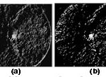Figure 3: Orientation map of the retinal image in Fig. 2(b). (a) Gray orientation map that is determined by using (4). (b) Binary orientation map that is determined by using (5). Click here to view full figure

 

For the retinal image in Fig. 1(a), Fig. 3(a) and (b) shows the determined gray orientation map and binary orientation map, respectively. As shown in Fig. 3(a), for retinal image pixels in quadrants I and III around the OD, the orientation map is a bit dark because the orientation of the line segment with the maximum variation usually lies between 1 and (n/2) + 1. However, for retinal image pixels in quadrants II and IV, the orientation map is bright because the orientation of the line segment with the maximum variation usually lies between n/2 and n. The binary orientation map in Fig. 3(b) further verifies such orientation pattern. The OD will then be located by using the orientation map to be described in the following.

Proposed circular convolution  

We use a line operator of 20 oriented line segments because line operators with more line segments have little effect on the orientation map. The line length p is set as follows:

p = k R                                                    (6)

where R denotes the radius of the central circular region of retinal images as illustrated in Fig. 1(a). Parameter k controls the line length, which usually lies between 1/10 and 1/5 based on the relative OD size within retinal images [25]. The use of R incorporates possible variations of the image resolution.

The specific pattern within the orientation map is captured by a 2-D circular convolution mask shown at the upper left corner of two peak images in Fig. 4.b. As shown in Fig. 4, the convolution mask can be divided into four quadrants, where the cells within quadrants I and III are set at−1, whereas those within quadrants II and IV are set at 1 based on the specific pattern within the orientation map. An orientation map can thus be converted into a peak image as follows:

where (x_o y_o ) denotes the position of the retinal image pixel under study. M(x, y) and    O(x, y) refer to the value of the convolution mask and the orientation map at (x, y), respectively. Parameter m denotes the radius of the circular convolution mask that can be similarly set as p.

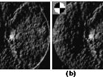Figure 4: Peak images determined by a 2-D circular convolution mask shown in the upper left corner. (a) Peak image produced through the convolution of the gray orientation map in Fig. 3(a). (b) Peak image produced through the convolution of the binary orientation map in Fig. 3(b). Click here to view full figure

For the orientation maps in Fig. 5(a) and (b), Fig. 6(a) and (b) shows the determined peak images. As shown in Fig. 4, a peak is properly produced at the OD position. On the other hand, a peak is also produced at the macula center (i.e., fovea) that often has similar peak amplitude to the peak at the OD center. This can be explained by similar brightness variation structure around the macula, where the image variation along the line segment crossing the macula center reaches the maximum, whereas that along the orthogonal line segment [similar to Lc and Lt in Fig. 1(b)] reaches the minimum. The only difference is that the OD center is brighter than the surrounding pixels, whereas the macula center is darker.

We, therefore, first classify the peaks into an OD category and a macula category, respectively. The classification is based on the image difference between the retinal image pixels at the peak center and those surrounding the peak center. The image difference is evaluated by two concentric circles as follows:

where I refers to the retinal image under study and d denotes the distance between the peak and the surrounding retinal image pixels. R1 and R2 specify the radius of an inner concentric circle and an outer concentric circle where R2 is set at 2 R1. Ni and No denote the numbers of the retinal image pixels within the two concentric circles. In our system, we set R1at    (p − 1)/2, where p is the length of the line operator. The peak can, therefore, be classified to the OD or macula category, if the image difference is positive or negative, respectively. Finally, we detect the OD by a score that combines both the peak amplitude and the image intensity difference that by itself is also a strong indicator of the OD

S(x,y) = P(x,y) (Diff(x,y) * (Diff(x,y) > 0))                            (9)

Where P(x,y) denotes the normalized peak image. The symbol * denotes dot product and Diff(x, y) > 0 sets all retinal image pixels with a negative image difference to zero. The OD can, therefore, be detected by the peak in the OD category that has the maximum score. For the example retinal image in Fig. 1(a), Fig. 5(a) shows the score image determined by the peak image in Fig. 4(b). It should be noted that the image difference is evaluated only at the detected peaks in practical implementation. The score image in Fig. 5(a) (as well as in Fig. 5(b), 9, and 10) where the image difference is evaluated at every pixel is just for the illustration purpose

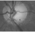Figure 5: OD detection. Score image by (9) for OD detection Click here to view full figure

 

Results And Discussion

The proposed method was implemented in MATLAB where runs needed on average 1.5min for each image on a laptop (Pentium(R) Dual-Core2 CPU and T4300@ 2.10GHz, 3.00 GB RAM 64-bit OS). The step by step output is shown in fig.6.(a)-(h)

The proposed method was evaluated both normal and abnormal retinal images using the subset of the DRIVE, STARE, and the success percentage was found to be 98.34% for all datasets(shown in table I).

 

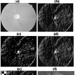Figure 6: (a)Input Image, (b)LAB – L Component, (c)Smooth Image, (d)Orientation map (e) Binary orientation map (f) Circular Convolution(g)Peak circular convolution mask(h) Detected Optic Disc Click here to view full figure

 

Table 1: Results

Dataset	No of Images tested	No of images failed	Success Percentage (%)
DRIVE	40	0	100
STARE	81	2	97.53
Total	121	2	98.34

The implemented binary orientation map is tested with our proposed method for all the 121 images of STARE and DRIVE datasets respectively it is achieve more comprehensive result when compare to other methods. Both data sets results are compared with other state of art methods (Fig.7a and b).

 

Figure 7: Comparison of the OD detection methods (a) STARE dataset (b) DRIVE dataset Click here to view full figure

 

Conclusion And Future Work

This paper presented a simple method for OD detection using binary orientation map. The proposed approach achieved better results as reported. An extension for this study could be as follows. region of interest would be the main objective of future work. Optic disc can be detected easily after segmentation. A myriad of Optic Disc detection methods are available.The image segmentation is the foundation for the retinal fundus images.  Efficient algorithms for segmenting the

The method which is compatible with the segmentation algorithm should be used. Diseases like Glaucoma and Diabetic Retinopathy are in rise and Optic Disc is an important indicator of these diseases. Hence the new methodologies to detect Optic Disc and the efficient use of already existing methods are the interest of future work.

Reference

1. Haseeb Ahsan, ”Diabetic retinopathy – Biomolecules and multiple pathophysiology” Diabetes & Metabolic Syndrome: Clinical Research & Reviews, Vol 9( 1), pp 51-54, 2015.
2. Peter H. Scanlon,”Diabetic retinopathy”, Medicine, Vol 43(1),pp 13-19, 2015.
3. David S.M. Burton, Zia I. Carrim “Angiographic Evidence of Peripheral Ischemia in Diabetic Retinopathy and the Risk of Impending Neovascularisation” Canadian Journal of Diabetes, Vol 39 (1), pp 14-15, 2015.
4. Ahmed M. Abu El-Asrar, Gert De Hertogh, Kathleen van den Eynde, Kaiser Alam, Katrien Van Raemdonck, Ghislain Opdenakker, Jo Van Damme, Karel Geboes, Sofie Struyf,”Myofibroblasts in proliferative diabetic retinopathy can originate from infiltrating fibrocytes and through endothelial-to-mesenchymal transition (EndoMT)”, Experimental Eye Research, Vol 132(1), pp 179-189,2015.
5. Sinthanayothin,J. F.  Boyce,  H.  L.  Cook,  and  T.H.Williamson.,”Automated  localization  of  Optic  Disc,fovea,and retinal  blood  vessels  from  digital  fundus  images”.,  Br  J Ophthalmol. 1999;83(8):902-10.
6. Arturo Aquino,  Manuel  Emilio  Gegúndez-Arias,  and  Diego Marín .,”Detecting the optic disc boundary in digital fundus images using  morphological,  edge  detection,  and  feature  extraction techniques”.,IEEE    Med.  Imag.,                Nov  2010.,vol.  29,  pp. 1860–1869.
7. Aliaa Abdel-Haleim  Abdel-Razik  Youssif,  Atef  Zaki  Ghalwash, and  Amr  Ahmed  Sabry  Abdel-Rahman  Ghoneim*.,”  Optic  Disc detection  from  normalized  digital  fundus  images  by  means  of  a vessels’  direction  matched  filter”, IEEE    Med. Imag.2008.,vol.27.,pp.11-18.
8. A.  Abdel-Ghafar,  T.  Morris,  T.  Ritchings,  I.  Wood.,”Progress towards automated detection and characterization of the  optic disc in glaucoma and diabetic retinopathy”., Med Inform Internet Med. 2007 ;32 (1):19-25.
9. Ashok  kumar,S.Priya,  Varghese  Paul.,”  Automatic  Feature Detection  in  Human  Retinal  Imagery  using  Bitplane  Slicing  and Mathematical  Morphology”.,  European  Journal  of  Scientific Research, Vol.80  No.1  (2012),  pp.57-67
10. F. Jeline, C. Depardieu, C. Lucas, D.J. Cornforth, W. Huang and M.J. Cree.,” Towards Vessel Characterisationin the Vicinity of the Optic Disc in Digital Retinal images”.,
11. ter  Haar,“Automatic  localization  of  the  optic  disc  in  digital colour  images  of  the  human  retina,” M.S.  thesis,  Utrecht University, Utrecht,The Netherlands, 2005.
12. Alireza Osareh,  Majid  Mirmehdi,  Barry  Thomas  and  Richard Markham.,“Comparison of colour spaces for optic disc localisation in  retinal  images”.,  Proceedings  of  the  16th  International Conference on Pattern Recognition . Suen, (eds.), pp. 743–746. August 2002.
13. Gopal Datt  Joshi,  Rohit  Gautam,  Jayanthi  Sivaswamy,    R. Krishnadas.,  “Robust  Optic  Disk  Segmentation  from  Colour Retinal Images” .,   Proceedings of the Seventh Indian Conference on  Computer  Vision,  Graphics and  Image  Processing,  pp.330-336 ACM New York, NY, USA ©2010.
14. Juan Xu,  Opas  Chutatape,  Eric  Sung,Ce  Zheng,  Paul  Chew  Tec Kuan.,  “Optic  disk  feature  extraction  via  modified  deformable model  technique  for  glaucoma  analysis”,  Pattern Recognition, 2006
15. Pallawala,Wynne Mong  Li  Lee, Guan  Au  Eong, “Automated Optic Disc Localization and Contour Detection  Using Ellipse  Fitting  and  Wavelet  Transform”,  Lecture  Notes  in Computer Science Vol. 3022 pp.139-151. , 2004,
16. Kenneth   Tobin,  Edward  Chaum,  V.  Priya  Govindasamya, Thomas  P.  Karnowskia,  Omer  Sezer., “Characterization  of  the optic  disc  in  retinal  imagery  using  a probabilistic  approach” Vol 82006;10pages;  DOI: 10.1117/12.641670.
17. Bowd C, Chan  K, Zangwill  LM, Goldbaum  MH, Lee TW, Sejnowski  TJ, Weinreb  ,  “Comparing  neural  networks and  linear  discriminant  functions  for  glaucoma  detection  using  confocal scanning laser ophthalmoscopy of the optic disc” Invest Ophthalmol Vis Sci.Vol. 43(11),pp3444-54,2002.
18. Niemeijer M, Abràmoff MD, van Ginneken B., “Fast Detection of the Optic  Disc  and  Fovea  in  Color  Fundus  Photographs”.,Med Image Anal. vol.13(6),pp859–870, 2009.
19. Marc Lalonde,  Mario  Beaulieu,  and  Langis  ,  “Fast  and Robust Optic Disc Detection Using Pyramidal Decomposition and Hausdorff-Based  Template  Matching”.,  IEEE  Trans.  Med.  Imag., 2001.,vol. 20, pp. 1193-1200.
20. STARE Project Website Clemson Univ., Clemson, SC [Online]. Available: http://www.ces.clemson.edu~ahoover/stare
21. Research section, digital retinal image for vessel extraction (DRIVE) database University Medical Center Utrecht, Image Sciences Institute,Utrecht, The Netherlands [Online]. Available: http://www.isi.uu.nl/Research/Databases/DRIV
22. Osareh, M. Mirmehdi, B. Thomas, and R. Markham, “Comparison of colour spaces for optic disc localisation in retinal images,” in Proc. Int. Conf. Pattern Recognit., vol. 1, 2002, pp. 743–746.
23. Tomasi and R. Manduchi, “Bilateral Filtering for Gray and Color Images,” in Proc. IEEE Int. Conf. Comp. Vis., 1998, pp. 839–846.
24. Mahfouz AE,  Fahmy    “Fast  localization  of  the  optic  disc  using  projection  of image  features”  IEEE  Transactions  on  Image  Processing , 2010;19(12):3285–9.
25. Lu   “Accurate  and  efficient  optic  disc  detection  and  segmentation  by  a  circular transformation”,  IEEE  Transactions  on  Medical  Imaging , 2011;30(12):2126–33.
26. Amin Dehghani, Hamid Abrishami Moghaddam,Mohammad-Shahram Moin,” Optic disc localization in retinal images using histogram matching”, EURASIP Journal on Image and Video Processing, vol.1(19),pp.1-11,2012.
27. Amin Dehghani, Mohammad-Shahram Moin and Mohammad Saghafi,” Localization of the Optic Disc Center in Retinal Images Based on the Harris Corner Detector”, Biomed Eng Lett Vol.2,pp.198-206,2012.
28. Kavitha, Duraiswamy, “An automatic retinal optic disc segmentation algorithm using differential windowing in the polar coordinate domain”, Australian Journal of Electrical Electronics Engineering, Vol. 10(1), pp.33-44,2013.
29. Avinash Ramakanth , R. Venkatesh Babu, “, Approximate Nearest Neighbour Field based Optic Disk Detection”, Computerized Medical Imaging and Graphics,Vol 38(1),pp 49–56,2014.
30. Neelam Sinha, Venkatesh Babu,” optic disk localization using l1 minimization”, IEEE International Conference on Image Processing, DOI: 10.1109/ICIP.2012.6467488,2012.

 

 

(Visited 390 times, 1 visits today)