Caroline Lall¹, Anushka Varshney¹, Sanjay Roka^1*, Ankur Maurya², Chandrakala Arya³, Manoj Diwakar¹, Prabhishek Singh²and JaiShankar Bhatt¹

¹CSE Department, Graphic Era Deemed to be University, Dehradun, Uttarakhand, India

²School of Computer Science, Engineering and Technology, Bennett University, India

³Graphic Era Hill University, Dehradun, Uttarakhand, India

Corresponding Author E-mail:sanjayroka05@gmail.com

Abstract

The brain is the main organ for regulating as well as coordinating all body processes. A brain tumor is defined as a growth of tissue that arises due to abnormal and uncontrolled cell division and is either malignant (cancerous) or benign (non-cancerous). The overall survival rate for primary brain tumors is approximately 75.2% so accurately and quickly diagnosing a brain tumor is essential. Depending on the method of diagnosis, traditional diagnosticians use a number of approaches that are often time-consuming and prone to human error. Therefore, computer-aided detection (CAD) approaches are becoming more appealing as a way to decrease human error. The ability to take medical Magnetic Resonance Imaging (MRI) scans and use independent computational models has evolved into a second approach to aid in brain tumor detection. In this research, deep learning techniques are used to classify brain tumors into three main categories like glioma, meningioma, and pituitary. A custom Convolutional Neural Network (CNN) model is created, and its performance is compared with two established architectures, that is, VGG-19 and ResNet-50. The VGG-19 model is appreciated for its simple yet powerful structure in image classification, whereas ResNet-50 is known for effectively managing deep networks through residual connections, preventing vanishing gradient issues. The classification accuracies were Custom CNN: 88.6%, VGG-19: 95.83%, and ResNet-50: 97.91%, demonstrating that ResNet-50 is most effective for automated brain tumor detection. ResNet-50 became famous for its capabilities to handle deep networks containing residual connections, a feature that helps mitigate vanishing gradient problems. The outcomes demonstrate how these frameworks, as well as special modifications, assist in attaining high diagnostic efficiency in detecting brain tumors

Keywords

Brain Tumor; CNN; Deep Learning; Detection; Machine Learning; MRI; Prediction; ResNet-50; VGG-19

Copy the following to cite this article: Lall C, Varshney A, Roka S, Maurya A, Arya C, Diwakar M, Singh P, Bhatt J. Comparison of CNN, VGG-19, and ResNet-50 Algorithm for Brain Tumor Detection. Biomed Pharmacol J 2025;18(October Spl Edition).

Copy the following to cite this URL: Lall C, Varshney A, Roka S, Maurya A, Arya C, Diwakar M, Singh P, Bhatt J. Comparison of CNN, VGG-19, and ResNet-50 Algorithm for Brain Tumor Detection. Biomed Pharmacol J 2025;18(October Spl Edition). Available from: https://bit.ly/4oQFBfx

Introduction

A tumor that is identified in the brain is characterized by uneven and unchecked proliferation in the brain cells or nearby regions. These tumors develop as a mass or cluster of dysfunctional cells that proliferate uncontrollably, potentially leading to significant health  During recent years, the need for precise, fast, and automatic analysis of medical images has led to greater efforts to produce automated systems for MRI analysis of brain tumors. Tumors are categorized as benign, i.e., non-cancerous, or malignant, i.e., cancerous. Globally, brain tumors affect nearly 700,000 individuals, with over 86,000 new cases reported in 2019 alone.

Detecting the early stages of a brain tumor can play a crucial role in improving patient prognosis. Conventional diagnostic methods frequently require significant manual effort, take considerable time, and are prone to human inaccuracies. Some tumors are benign and pose minimal risk, while others may be aggressive and life-threatening if not detected promptly. MRI, ie, Magnetic Resonance Imaging, and CT, i.e., Computed Tomography scans are mostly employed to detect abnormalities in brain structure, including tumors.

Among these, MRI is generally preferred due to its superior soft tissue contrast and ability to provide more detailed and clearer images. As a result, MRI-based diagnostics are now the focus of much research and medical exploration. 

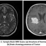Figure 1: Sample Brain MRI Scans: (a) Structure of Normal Brain (b) Brain showing presence of Tumor Click here to view Figure

As shown in Figure 1, by comparing the MRI scans of a normal brain (A) and a tumor brain (B), manual analysis of such scans is not as easy. Noise and artifacts introduced during the imaging process, together with the brain structure’s complexity, complicate the interpretation by radiologists, making it accurate and reliable only to a certain extent. Besides, manual analysis is dependent on the experience and professional judgment of the radiologist, which may bring variability and errors to the diagnosis. The increased size of the medical datasets’ images further exacerbates the problems with manual inspection. This implies that computer-aided diagnostic (CAD) systems need to arrive in a position to assist the clinicians, especially when it comes to tumor detection in the brain. One of the principal components of these systems is pre-processing MRI scans to minimize noise and intensity in homogeneities so that they are more convenient for machine examination and the likelihood of detecting minuscule abnormalities that are too small for the human eye to see. In another  A deep learning framework was developed to efficiently detect and segment brain tumors using a CNN. Among the many deep learning techniques, Convolutional Neural Networks (CNNs) have demonstrated extraordinary effectiveness in visual pattern recognition tasks. CNNs have been applied extensively in applications ranging from facial recognition and image classification to medical diagnostics and environmental data analysis. In medical imaging—especially for brain tumor detection—CNNs have persistently outperformed classical machine learning algorithms with higher accuracy and precision. While traditional machine learning models can provide quicker training times, they tend not to have the deep feature extraction ability that comes with CNN designs.

The primary objective is to create an automated model that can detect brain tumors from MRI scans. This research aims to compare the two leading architectures—VGG-19 and ResNet-50—to analyze their performance in tumor classification. Aside from these pre-trained models, the paper also delves into the creation and deployment of a custom CNN. The custom CNN is specially crafted for tumor classification, making use of bespoke convolutional layers and pooling steps. Unlike the pre-trained models, the custom CNN is tuned to the problem, possibly increasing accuracy and mitigating overfitting for the particular dataset. By the outcomes of VGG-19, ResNet-50, and the resultant custom CNN. This research aims to provide useful insights into which model provides the most effective classification, performed based on parameters such as accuracy, precision, recall, and F1-score. The results of this research would be very helpful to health practitioners in more precisely and efficiently diagnosing brain tumors, thus making more effective treatment and patient care decisions.

The paper is organized as follows: Section II is the literature survey and the current methodologies. Section III outlines the proposed system architecture and the methodology framework. Section IV explains the model development and implementation process and the experimental results. Finally, Section V has the summary of detection and recommendations of directions for future research.

Literature Review

Different works have addressed the problem of classifying brain tumors from the scans produced by MRI by using novel techniques as well as deep learning architectures. In a significant paper, a stacked classifier model was introduced based on transfer learning, known as VGG-SCNet. This model used pre-trained networks, that is, VGG-19, to extract high-level features from MRI images, and the features were classified using another classifier. The method showed promising performance with a high F1-score. Hybrid and ensemble machine learning techniques were also investigated by the study to enhance classification accuracy further, which brought out the benefits of less manual feature extraction, thereby automating the detection of tumors. The union of transfer learning and stacked classification models has proved to be good in performance and efficiency for several medical imaging tasks.

In another research, a deep learning framework was developed to efficiently detect and segment brain tumors using a CNN. The suggested framework first utilized a CNN for tumor presence detection. Subsequently, segmentation methods, such as autoencoders and tumor regions, were effectively detected using K-means clustering in the MRI scans. This blended methodology of using unsupervised learning (K-means) and deep learning (autoencoders) assisted in obtaining cleaner segmentations by filtering out noise, thus minimizing the need for manual intervention and speeding up the diagnosis process. A thorough analysis of brain tumors through images was performed  with emphasis on the BRAMSIT MRI dataset that comprises 319 MRI brain scans. When used for image classification and feature extraction methods in a series of experiments, this dataset was utilized. The investigation set out to benchmark methods based on classification performance so as to provide valuable groundwork for future work in the field. The findings of this analysis revealed that HOG and LBP were some of the feature extraction methods used, which were very efficient in differentiating healthy and tumorous brain tissues and providing rich insights for detection systems. Early detection greatly improves the chances of successful intervention and can prevent the tumor from pressing on vital brain structures or metastasizing to adjacent

presented a novel method for microscopic-level brain tumor classification by incorporating a 3D CNN structure. The architecture of the model was tailored to process volumetric data, and the fine-grained spatial features were obtained from MRI scans. The obtained features were processed by a pre-trained CNN, and for final classification, a feed-forward neural network was employed. This multi-layered design assisted in enhancing the capability of the model to identify and classify types of tumors at a finer level, providing an enhancement in accuracy to classify systems depending on the tumor.  An empirical study was carried out to explore the importance of feature selection in medical image classification. The study involved extracting tumor-related features and grouping them into distinct sets. To determine the most optimal approach, several models of ML were tested to find the powerful feature set and classifier combination for achieving the highest accuracy. This approach, while generally applied to the prediction of outcomes for other illnesses, was equally pertinent to brain tumor prediction. The research highlighted the importance of choosing the most informative features in order to increase the accuracy of predictive models, particularly when dealing with heterogeneous and high-dimensional data.

A segmentation technique employing Fuzzy C-Means (FCM) clustering algorithms was presented  for localizing tumors within MRI scans. Once images were segmented, standard classifiers were applied to perform classification operations like K-Nearest Neighbors (KNN), Logistic Regression (LR), MLP, Random Forest (RF), Naive Bayes (NB), and SVM. Out of all, the SVM model had the highest classification to identify accuracy. 92.51% was realized, which shows excellent performance in medical image classification. The success of the SVM model in this case highlights the importance of selecting appropriate classifiers that are appropriate for the nature of the data and the intended application. A novel model, known as the Artificial Convolutional Neural Network (ACNN), was proposed  to automatically identify tumors in brain MRI images. The ACNN model was created to classify images into binary classes: tumor-present and tumor-absent. The model achieved a test accuracy – 88.25% and an evaluation accuracy – 96.7%, demonstrating its strength and practicality. These findings highlight the accuracy of CNN-based models in medical image classification with fairly high precision, which qualifies them for use in clinical scenarios where precision is most important. Finally, an ultra-light CNN model was presented  for discriminating between healthy and tumorous MRI scans. The model used a lightweight architecture with only three convolution layers, combined with simple preprocessing methods. Notably, the simple model was still able to deliver a high 96.08% accuracy and an F1-score of 97.3% after a mere 35 training epochs. This shows that even shallow CNN models, properly optimized, are capable of achieving highly accurate performance with low computational overhead.

Past works also relied upon fewer datasets spanning low diversity, limiting the models’ generalization capability in clinical settings. In addition, hybrid or attention-based architectures that would improve feature extraction and minimize the cases of overfitting were not addressed in many studies. To overcome such limitations, future research should also consider lightweight models (e.g., EfficientNet, MobileNetV3) and transformer-based models (e.g., Vision Transformer (ViT)), which could offer improvements to the performance-efficiency relationship. Transfer-learning approaches, which incorporate attention mechanisms or multi-modal MRI data, may also provide improvements in robustness and accuracy of diagnostic data. Additionally, explainable AI may provide greater veracity by offering meaningful and accessible tumor predictions and intervention in clinical decision-making. Furthermore, advancing datasets, improving pre-processing pipelines, and testing on real-time medical modalities will also improve the practicality and validity of study applications in varying contexts of the healthcare ecosystem.

Materials and Methods

This work largely uses Convolutional Neural Networks (CNNs) as the foundational algorithm for brain tumor detection, leveraging the proven success of CNNs in image classification problems, particularly in medical imaging. The topic of this paper is to perform a comparative analysis of two popular deep learning models—VGG-19 and ResNet-50. Apart from these very popular models, an in-house developed CNN model is also suggested. The reason behind the addition of the proprietary model is to establish if an architecture can be created with more precision and accuracy in detecting tumors. The methodology followed here is structured in the form of an extensive, multi-step process that comprises main steps such as dataset gathering, image preprocessing, data augmentation, model training, and subsequent performance evaluation. Flowchart 3.1 is a step-by-step and graphical representation of the entire adopted pipeline for brain tumor detection using the implementation of deep learning strategies. This is initiated with the initial installation and configuration of the development environment. Here, all the libraries, dependencies, and frameworks that are needed to install a stable and functional working environment for the implementation of machine learning models are installed and initialized. Once the environment is created, the MRI scan dataset is uploaded into the system, which represents the beginning of the data preparation phase. Perhaps the most critical component of this pipeline is the image preprocessing step, which guarantees that the raw MRI data are being transformed into a format that is compatible with deep learning algorithms. This involves resizing each image to a standard fixed size to maintain uniformity in the dataset.

Standardization is required to ensure that the model is given consistent input shapes, which is a prerequisite for successful training. Furthermore, pixel normalization is performed to normalize image intensities, which helps to accelerate model convergence and enhance learning stability. The second essential preprocessing step is labeling each image to indicate whether or not there is a brain tumor. By tagging, supervised learning is eased since the model is equipped with unequivocal targets for categorization. All of these steps combined are essential to reorganize unstructured and heterogeneous medical imaging data into a structured, normalized form that can be processed efficiently by deep learning algorithms, offering a solid foundation for accurate tumor classification.

Besides the enlargement of the size and variance of the training data set, many of the data augmentation methods are utilized. These are comprised of many different operations such as image rotation, flipping, zooming, and shifting. Data augmentation provides an added variation in the training data so the model becomes improved in terms of generalizing new, unseen images. This reduces the likelihood of overfitting and makes the model stronger in being adaptable in real-world scenarios. The core of the workflow is in training and evaluating three standalone CNN-based models, like CNN, VGG-19, and ResNet-50. The models are trained using the preprocessed and augmented datasets with the ability to learn to distinguish MRI scans between the presence or no presence of tumors. The trained models are put through a rigorous test to check their performance and reliability. Test metrics used include accuracy (showing the general accuracy of the predictions), precision (showing the proportion of correctly predicted tumors that are actually tumors), recall (showing the capability of the model in recognizing actual tumor cases), and the F1-score (harmonic mean of precision and recall). These measurements provide a numerical basis for quantitatively comparing the performance of the different architectures.

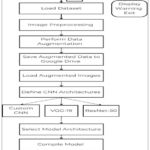Figure 2: Key Steps for Brain Tumor Detection Click here to view Figure

Brain Tumor Image Preprocessing

Image preprocessing is an important step before training deep learning models using MRI scans. Since the raw MRI images within the dataset will be of different resolutions, aspect ratios, and possibly contain irrelevant black borders or noise, standardization becomes a necessary step to provide uniform input to the models. To solve these problems, the preprocessing is done through the Python Imaging Library (PIL) by importing the Image module from PIL import Image. The library facilitates strong image manipulation abilities with basic simplicity and flexibility. Because both the VGG-19 and ResNet-50 architectures expect the input images to be of 224 × 224 pixel size, each of the MRI scans is resized accordingly. However, directly resizing the images can lead to distortion, particularly in cases where the original images have non-square dimensions. To preserve the anatomical integrity of the brain structures, the preprocessing pipeline includes an important step of cropping the region of interest—specifically, the brain area—from the scans.

Cropping is performed manually or through PIL-based techniques by identifying the area with significant pixel intensity variation and excluding background regions. This approach helps isolate the brain region, removes unnecessary black padding, and ensures that the model’s attention remains focused on the meaningful parts of the image. After cropping, each image is carefully resized to 224×224 pixels. To further enhance consistency across the dataset, pixel values are standardized by scaling them within a range of 0 to 1. This standardization aids in balancing the process of training and ensures that the learning algorithm is not biased due to varying brightness or contrast across different scans. This entire preprocessing pipeline ensures that the MRI scans are not only standardized in terms of size and format but also refined to emphasize the regions most relevant for tumor detection. As a result, the deep learning models are better equipped to learn and distinguish features associated with different types of brain tumors. Figure 2 illustrates an example of a brain MRI image after undergoing the complete preprocessing procedure.

Data Augmentation

Considering the limited size of the available MRI dataset, the major concern is overfitting, where the model shows high performance on data that needs to be trained but struggles to adapt to new, undetected images. To resolve the above problem, data augmentation methods are used to artificially expand the dataset. Augmentation of data plays a crucial role in workflows of deep learning, especially when dealing with small datasets, as it introduces variability and diversity into the training data without requiring additional collection of the data. Data augmentation techniques like rotation, flipping, zooming, and shifting artificially expand datasets, helping reduce overfitting and improve   Figure 3 demonstrates the difference between a cropped and preprocessed MRI Image. In this study, a series of commonly used image transformation techniques is applied to the existing brain MRI scans to generate modified versions of the original images. These transformations include random rotations to simulate different orientations of the brain, horizontal and vertical flips to account for symmetry variations, shifts in width and height to mimic positional changes, zooming to simulate different imaging distances, and shearing to apply slight geometric distortions.

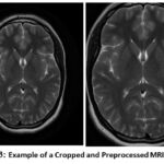Figure 3: Example of a Cropped and Preprocessed MRI Image Click here to view Figure

Each transformation slightly alters the image while preserving the underlying features relevant to tumor detection. This augmentation process assists the model in learning more abstract and resilient patterns instead of memorizing the unique details of a single image. By presenting the model to a greater variety of image variations, it is improved at managing real-world clinical data, which in practice may contain variations in scanning angle, lighting, and patient position. Therefore, the application of data augmentation considerably improves the model’s ability to make accurate predictions on different MRI scans, finally improving its reliability in real diagnostic use.

Proposed System

This work suggests a brain tumor detection model that uses deep learning models to analyze MRI images. In particular, the model uses pre-trained CNNs, i.e., VGG-19, along with ResNet-50, and presents a custom CNN architecture designed for effective tumor classification. The models are evaluated and compared based on accuracy, recall, precision, as well as F1- score. This is done to determine their performance and in identifying accurately identify tumors in brain MRI images.

Convolutional Neural Network (CNN Architecture)

In this case, a specialized Convolutional Neural Network (CNN) architecture was created for tumor categorization that exists in the brain using scans conducted via MRI. The model starts with a series of convolutional layers that utilize a stride of 2 for down-sampling in place of max pooling. This method preserves more spatial features while at the same time decreasing the dimensionality. In particular, the architecture includes 3 convolutional layers with filter sizes of 32, 64, and 128, each of which is followed by batch normalization to boost training stability and speed. Following the convolutional blocks, a global average pooling layer is used to reduce the maps of features into a dense vector to prevent the risk of overfitting. This is succeeded by a 128-neuron dense layer and ReLU activation to store high-level representations, and also by a 30% dropout layer to again prevent overtraining. The output layer has a softmax activation function for classifying the input images into four tumor classes.

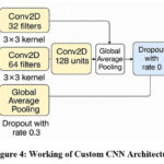Figure 4: Working of Custom CNN Architecture Click here to view Figure

Figure 4 shows the working of the custom CNN Architecture. The model is subsequently built using the Adam optimizer. Additionally, sparse categorical cross-entropy loss is used to train it, which is appropriate for multi-class classification problems. This bespoke CNN is light relative to large pre-trained models and is thus efficient without a loss of classification accuracy on brain MRI datasets. Through training the custom CNN in conjunction with VGG-19 and ResNet-50, this work seeks to determine if a designed, lighter framework can be equally effective as, or even superior to, these established models in terms of efficiency and resource utilization.

VGG-19 Architecture

VGG-19 is a deep convolutional neural network model from the Visual Geometry Group of the Oxford University. It was popular due to its plain and robust design, which is based mainly on the philosophy of stacking many convolutional layers with small-sized 3×3 filters. This simplicity of design, coupled with an in-depth structure of 19 weight layers, renders VGG-19 not only highly performing but also easy to use, adopt, and fine-tune for a broad spectrum of image classification tasks. In the context of this research, VGG-19 is used as a base model for brain tumor detection tasks. The model is instantiated with pre-trained weights that have been downloaded from the ImageNet database, which contains a very large image repository of more than one million images labeled and annotated for 1,000 object categories that vary widely. Relying on the pre-trained weights, the model leverages previously learned visual features such as patterns, texture, and edges that are presumably transferable to other applications such as medical imaging. This transfer learning method has a considerable decrease in the computational expense and time needed, as it does not require training a deep neural network from scratch. To modify VGG-19 for the particular problem of brain tumor classification, the include_top=False parameter is used during model initialization. This configuration leaves out the usual top layers of the VGG-19 model, namely the fully connected top layers intended initially for multi-class ImageNet classification of classes. These top layers are stripped so that the integration of personalized classification layers, particular to the binary problem at hand, detection of presence or absence of a brain tumor in an MRI scan can be added.

Omitting the highest layers, the model now acts as a feature extractor that only works on discovering the low-level features of shapes, edges, and textures, and also the mid-level patterns like the object parts, all the significant ones, while trying to distinguish various brain tumors found in MRI scans. Following the extraction, another classification head is appended to the network. This is then followed by a flattening layer to map the multidimensional feature maps to a one-dimensional vector, followed by one or more dense layers that discover complicated relations among the features. The last dense layer consists of neurons corresponding to the number of target classes — for us, four — and each corresponds to a different kind of brain tumor. This method falls under the transfer learning category, where a model trained for one task is utilized to address another, but similar task. The pre-trained VGG-19’s convolutional layers are first frozen, i.e., their weights remain constant during training. This means that the learned low-level features are not lost. Subsequently, selective fine-tuning is realized by unfreezing deeper layers so that the network can update its internal representations to suit the new dataset better, improving performance. The working of the VGG-19 architecture is shown in Figure 5.

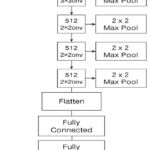Figure 5: Working of VGG-19 Architecture  Click here to view Figure

Key Features of VGG-19

Uniform Filter Size

Uses 3×3 convolutional filters across the network with a stride of 1 and padding, ensuring spatial resolution is maintained and permitting fine-grained feature extraction.

Max-Pooling for Down-sampling

Adds 2×2 max-pooling layers at fixed intervals to decrease feature map dimensionality, lower computational burden, and avoid overfitting.

Transfer Learning with Pre-Trained Weights

Leverages pre-trained weights from the ImageNet dataset, allowing the model to transfer visual feature knowledge like edges, textures, and shapes to medical imaging tasks, thus saving time and resources.

Top Layer Removal (include_top=False)

The default classification layers are omitted during model initialization to enable integration of custom classification layers that are specifically designed for brain tumor detection.

Custom Classification Head

Added with a flatten layer, then dense layers, with a final output layer of 4 neurons (for four types of tumors), enabling it to do multi-class classification on MRI brain images.

Frozen and Fine-Tuned Layers

The convolutional base is first frozen to preserve learned features, then selective unfreezing of deeper layers for fine-tuning, improving performance on the new dataset.

ResNet-50 Architecture

ResNet-50 model utilization was done through transfer learning for brain tumor classification. ResNet-50 (50-layer Residual Network) is designed as a deep CNN model introduced by Microsoft Research and is known for its use of residual learning to ease the training of very deep networks. In traditional deep networks, with the increase in the number of layers, problems like vanishing gradients may cause performance degradation. ResNet solves this by introducing shortcut connections (also referred to as skip connections), which enable the network to learn residual functions rather than straightforward mappings. These shortcut paths facilitate the training of significantly deeper architectures by enabling gradients to flow through the network without vanishing, thus improving convergence and accuracy. The ResNet-50 architecture contains convolutional layers, the ReLU activation function, identity blocks, as well as batch normalization. Here, convolution blocks are arranged systematically. It contains approximately 23 million parameters and is divided into multiple stages, with each stage containing several building blocks. Each block contains convolutional layers with shortcut connections directly adding the input to the output, as shown in Figure 6.

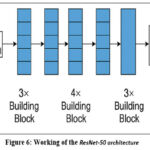Figure 6: Working of the ResNet-50 architecture Click here to view Figure

In this setup, the ResNet-50 model was initialized with the previously trained weights of ImageNet, weights = ‘imagenet’, which are also configured with include_top = False, which excludes the original fully connected layers. This modification enables the model to function as a feature extractor for MRI brain images. After the ResNet-50 base, custom fully connected (dense) layers were added to adapt it specifically for the brain tumor classification task (with the appropriate number of output classes). Optionally, the base ResNet-50 layers can be frozen to retain their learned low-level feature mappings, while the new dense layers are trained on the MRI dataset, improving generalization and speeding up training. Using ResNet-50 helps in achieving high classification accuracy because it is deep enough to capture complex image features while avoiding overfitting and degradation problems typical in very deep networks. Figure 7 shows a pie chart using ResNet-50.

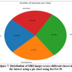Figure 7: Distribution of MRI images across different classes in the dataset using a pie chart using ResNet-50 Click here to view Figure

Classification

For the classification task, models like VGG-19, ResNet-50, and a custom CNN architecture are implemented and trained on the dataset, which is augmented. Both the VGG-19 as well as ResNet-50 models are well-established deep learning models that are recognized for their capability to extract detailed, multi-level features from images. VGG-19, a 19-layer architecture, is prized for its simplicity in layout and its use in classifying images. ResNet-50, on the other hand, uses residual connections to solve the vanishing gradient problem in deeper neural networks, allowing training to occur efficiently even with greater depth.

The two networks mentioned, as well as a specialized CNN architecture that was created to check if a dedicated network can provide improved results for brain tumor image classification, are used. The proprietary CNN includes layers that are specifically tailored to the kind of image features found in MRI scans, e.g., small kernel size convolutional layers and batch normalization for better convergence. Through the utilization of a smaller, more efficient network, the proprietary CNN seeks to offer a balance between performance and computational functionality, which makes it appropriate for application in real-time medical applications. This project entails the construction of a bespoke Convolutional Neural Network (CNN) to suit the classification of tumors in the brain that are contained therein using MRI scans. Rather than max pooling used in the past, the model utilizes strided convolutions (stride of 2) for down-sampling, allowing spatial information to be preserved while decreasing feature map size. The network contains 3 convolutional layers with 32, 64, and 128 filters, subsequently followed by batch normalization to promote stability and efficacy during training.

After the convolutional layers, to reduce the feature maps into a compact vector, a global average pooling layer is employed, which serves to reduce the chance of overfitting. This is succeeded by a fully connected layer comprising 128 neurons with ReLU activation, designed to capture abstract patterns. To decrease model over complexity, a layer of dropout with having 30% rate is applied. The resultant layer employs an activation function based on softmax to categorize the MRI images given as input towards one of four tumor types. The model utilizes the Adam optimizer for compilation and is trained with the help of sparse categorical cross-entropy loss, which is suitable for multi-class classification tasks. This custom CNN is lightweight compared to large pre-trained models, making it efficient while maintaining good classification performance on brain MRI datasets. By training the custom CNN alongside VGG-19 and ResNet-50, this study aims to assess whether a tailored, lighter architecture can perform comparably to or outperform these well-established models, especially with regard to both efficiency and resource consumption. Figure 8 shows the Architecture of MRI-based brain Tumor Classification.

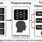Figure 8: Architecture of MRI-Based Brain Tumor Classification Click here to view Figure

The classification models are trained using an appropriate optimizer (such as Adam or SGD) and an ideal loss function, particularly for binary categorization, such as binary cross-entropy. Here, model performance is evaluated by evaluating metrics like accuracy, F1-score, precision, and recall for both training as well as validation sets. These metrics help evaluate and analyze the functionality of the VGG-19, ResNet-50, including custom CNN models, identifying the most effective one for the detection of brain tumors. Figure 9 shows the Classification of Brain Tumor MRI. 

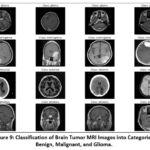Figure 9: Classification of Brain Tumor MRI Images into Categories: Benign, Malignant, and Glioma. Click here to view Figure

Experimental Setup Result and Analysis

Brain MRI Dataset

The dataset utilized was acquired from Kaggle, containing 254 scans of MRI of the human brain. Further, these scans are grouped into four different classes, such as glioma, no tumor, pituitary tumor, and meningioma. Different categories show a particular medical condition, enabling the deep learning models to identify unique features for the precise classification of different brain tumor types. This multi-class approach is especially useful for training models to differentiate between various tumor types and normal brain tissue. Due to the heterogeneous nature of the dataset—varying in image dimensions, formats, and quality—a comprehensive preprocessing pipeline was implemented. This process involved resizing all images to a standardized resolution to ensure consistency, converting them into a uniform supported format that meets the model’s input demands, and applying normalization techniques to scale pixel intensity values. These steps are crucial for enhancing computational efficiency and ensuring stable model convergence during training. An illustrative sample of the pre-processed images is presented in Figure 10, showcasing the visual differences between the classes.

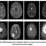Figure 10: Brain MRI Samples from Dataset: (a) Non-tumorous (normal) brain images; (b) Tumorous brain images. Click here to view Figure

Experimental Setup

Mount Google Drive for Accessing the Dataset

Mount Google Drive to access files stored in it. Check GPU availability using the nvidia-smi command to ensure GPU usage for model training.

Dataset Path Setup and Image Collection

Define the path to the dataset. Use glob to gather image file paths from the dataset directory recursively for various image formats (jpg, jpeg, png, etc.). Display the total number of images found.

Data Augmentation Setup

Use ImageDataGenerator from Keras to apply methods for augmenting data like rotation, shifting, shearing, zooming, and horizontal flipping. The Keras guide explains the concept of how transfer learning reutilizes a pre-trained model’s learned features for a new task, especially useful when data is

Load and Preprocess Images

Load images from the dataset folder, resizing them to 128×128 pixels and converting to grayscale. Create a NumPy array for the images and labels.

Apply data augmentation and generate new augmented images, then combine them with the original data. Save the images, labels, and class names to Google Drive.

Data Loading for Model Training

Load the preprocessed image and label data from Google Drive for model training. Display the number of images, labels, and class names.

Visualization of Sample Images

Select a subset of 4 images per class for visualization. Display the selected images along with their respective class names.

Class Distribution Visualization

To better understand the dataset, generate a pie chart that visualizes the proportion of samples belonging to each class (e.g., glioma, meningioma, pituitary, and no tumor).

This helps identify any class imbalances that could affect model performance and inform the need for strategies like class weighting or data augmentation.

Model Training and Splitting of Data

Divide the dataset into training and testing subsets, commonly using a 90:10 split ratio.

Ensure that the split enables the model to recognize patterns during training while preserving a separate subset for evaluating generalization performance.

Build Convolutional Neural Network (CNN)

Design a custom CNN architecture using TensorFlow/Keras. Include convolutional layers to extract features, which is succeeded by global average pooling to reduce data dimensions. Incorporate batch normalization layers to stabilize and accelerate training, and dropout layers to minimize overfitting.

The model should conclude with dense layers ideal for categorization. The execution of the model is done with the help of the Adam optimizer, followed by categorical cross-entropy loss, which is suitable for the classification of multi-class problems.

Using Pretrained Models (ResNet50, VGG19)

Apply transfer learning by utilizing pretrained models such as ResNet50 and VGG19. Freeze the convolutional base layers to retain learned features from ImageNet, and append custom dense layers tailored to the target brain tumor classification task.

This approach enhances performance, especially when working with limited medical imaging data, by leveraging previously acquired knowledge.

Model Training

Train the CNN and transfer learning models using the model.fit() method, which involves setting parameters like size of the batch, the total number of epochs, in addition to a validation split (example 10%) to track the model’s productivity on the data that is not seen during training.

Save as well as Load the Model which is Trained

Once training is done, then preserve the model to a designated directory, such as Google Drive, using the model.save() method. This facilitates reuse without retraining.

Later, load the model using load_model () to make predictions or resume training as needed.

Testing and Model Evaluation

Evaluate the trained model on the test dataset with the help of metrics like accuracy, precision, recall, and F1 score.

Create a confusion matrix to determine how well the model distinguishes between different tumor types and identify common misclassifications.

Visualize Training History

Generate plots visualizing training as well as validation accuracy and loss across each epoch.

These visualizations help assess whether the model is learning effectively, overfitting, or underfitting. They are crucial for model diagnosis and optimization.

Model Prediction on New Images

Implement a custom function to classify unseen ­MRI images. This involves loading an image, resizing it to the required input shape, normalizing pixel values, and utilizing the model, which is trained for generating predictions.

The predicted class label is then returned for interpretation.

Display Random Test Predictions

Randomly select a set of test images and display them alongside their true and predicted labels.

Present these images in a grid format for visual comparison. This qualitative analysis provides an understanding of how the model is performing in real-time situations.

Ablation Study

Impact of Convolution and Batch Normalization

In the custom CNN model, we increased Conv2D and Batch Normalization layers so the model gradually becomes deeper, which enables the model to record more sophisticated and complex patterns from the images given as input. The initial convolutional layers focus on identifying basic elements such as borders and structures. On adding more layers, the model begins to recognize more sophisticated patterns such as shapes, object parts, or, in the case of MRI scans, different tissue structures and tumor boundaries.

Each time we apply a convolution with a stride of 2, the spatial dimensions of the image (width and height) are reduced by half, while the number of feature channels typically increases. However, as the depth increases, the model’s complexity also grows, leading to a greater risk of overfitting if not enough data is available for training.

The model may memorize training images rather than generalizing to unseen data. Furthermore, deeper networks require more computational resources, more memory, and longer training times. At the third layer, the model achieves only 67.61% training and 70.9% testing accuracy, indicating under-fitting due to limited feature extraction. Increasing to four layers improved the result from 73.5% to 77.3%. At five layers, there was a slight drop from 71.6% to 75.3% due to mild overfitting. The six-layer model showed the best performance that is reaching 83.0% training and 88.6% testing accuracy. On adding a seventh layer, it reduced the performance was reduced from 64.2% to 67.4%, which happened due to overfitting or vanishing gradients. Overall, the six-layer CNN overcame deeper models, showing 17% improvement in testing accuracy over the shallowest network. This shows that moderate network depth yields optimal feature learning and stable generalization. Table 1, given below, shows the Impact of Conv2D Layer Depth on Model Accuracy and Generalization Capability.

Table 1: Impact of Conv2D Layer Depth on Model Accuracy

Conv2D Layers	Training Accuracy	Testing Accuracy	Explanation
3	67.61%	70.9%	Model too shallow; insufficient feature extraction; under-fitting.
4	73.5%	77.3%	Slightly deeper model captured better features; improved learning.
5	71.6%	75.3%	Minor overfitting starts; model learning improves, but generalization weakens slightly.
6	83.0%	88.6%	Optimal model depth; best balance between feature learning and generalization; minimal overfitting.
7	64.2%	67.4%	Model becomes too complex; overfitting or vanishing gradient issues; poor generalization and unstable training.

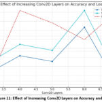Figure 11:  Effect of Increasing Conv2D Layers on Accuracy and Loss Click here to view Figure

Without architectural innovations like skip connections (used in ResNet), very deep models might also suffer from vanishing gradients. Batch normalization partly addresses this by stabilizing the learning process and helping gradients flow better through the network. Nonetheless, after a certain depth, simply stacking convolutional layers is not enough; the network would benefit from smarter design choices like residual blocks or dense connections to maintain performance and stability. As the number of layers are increased, it makes the model to grasp more strong as well as sophisticated features, potentially enhancing classification performance, but it also introduces challenges related to overfitting, training difficulty, and computational cost, which need to be carefully managed for successful deep model development. Figure 11 represents the effect of increasing Conv2D Layers on Accuracy and Loss via a graph.

Impact of Loss Function

The table shown below presents a comparison of model performances using different combinations of loss functions and architectures, evaluated based on their classification accuracies. Two loss functions — Sparse Categorical Crossentropy and Categorical Crossentropy — were paired with two different models: a basic Conv2D-based CNN and a deeper ResNet50 network. Loss functions are crucial during training as they measure the difference between the model’s predictions and the true labels, guiding the learning process. Here, the model uses this feedback to adjust its parameters and minimize the loss, ultimately aiming to enhance its accuracy. Sparse Categorical Crossentropy is typically applied when class labels are provided as integers (e.g., 0, 1, 2), while Categorical Crossentropy is used when labels are one-hot encoded vectors (e.g., [1, 0, 0] for class 0). Although both are intended for multi-class classification tasks, their usage depends on the format of the labels. Figure 12 shows Model Accuracy Comparison Based on Loss Function via a bar graph.

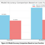Figure 12: Model Accuracy Comparison Based on Loss Function Click here to view Figure

The table shows that both models performed better with Sparse Categorical Cross-entropy compared to Categorical Cross-entropy. Specifically, the Conv2D model attained an accuracy of 67.8% with Sparse Categorical Crossentropy, significantly higher than the 52.68% accuracy obtained with Categorical Crossentropy. Similarly, the ResNet50 model, being more complex and deeper, achieved 88.68% accuracy with Sparse Categorical Crossentropy, whereas its performance dropped to 54.84% with Categorical Crossentropy. Several important insights can be drawn from these findings. First, the ResNet50 model consistently outperformed the simpler Conv2D model, regardless of the loss function used. This is expected, given ResNet50’s deeper and more sophisticated architecture, which is better suited for complex image classification problems. Secondly, the selection of the loss function greatly impacted the model’s performance. The superior results with Sparse Categorical Cross-entropy indicate that the dataset labels were likely in integer format, making this loss function more appropriate. In summary, the comparison highlights that both the selection of model architecture and the appropriate loss function are crucial for achieving high classification accuracy. The combination of a deeper network like ResNet50 with the correct loss function (Sparse Categorical Crossentropy) led to the highest accuracy of 88.68%, while simpler models or mismatched loss functions resulted in lower performance. Table 2 shows the Effect of Loss Functions on Model Performance and Accuracy for Conv2D and ResNet-50 Architectures.

Table 2: Impact of Loss Functions on Model Performance and Accuracy

Loss Function	Model	Accuracy
Sparse Categorical Cross-entropy	Conv2D	67.8%
Sparse Categorical Cross-entropy	ResNet-50	88.68%
Categorical Cross-entropy	Conv2D	52.68%
Categorical Cross-entropy	ResNet-50	54.84%

Analysis of VGG-19 vs ResNet-50 Model Performance

The crucial models used in this paper, VGG-19 in addition to ResNet-50, model’s performance is assessed through widely used classification analysis, like – accuracy, F1-score, precision, and recall. The tabular representation below shows the comparison between VGG-19 and ResNet-50 models for brain tumor classification, based on both training and testing metrics. During training, ResNet-50 slightly outperforms VGG-19 with a higher accuracy (98.46% vs. 96.93%) and F1-score (98.50% vs. 97.05%), indicating better overall learning capability and more precise predictions. It also maintains perfect recall and slightly higher precision. In the testing phase, which reflects real-world generalization, ResNet-50 again shows superior performance with a 97.91% accuracy and 97.95% F1-score, compared to VGG-19’s 95.83% accuracy and 96.0% F1-score. These results suggest that ResNet-50 not only learns better during training but also generalizes more effectively on unseen data, making it a more reliable and robust model for the detection of brain tumors, as shown in the comparison Table 3.

Table 3: Comparison between VGG-19 and ResNet-50 Architecture

	VGG-19	ResNet-50
Training Performance	Accuracy:  96.93%Precision:  94.28%Recall:  100%F1-Score:  97.05%	Accuracy:  98.46%Precision:  97.05%Recall:  100%F1-Score:  98.50%
Testing Performance	Accuracy:  95.83%Precision:  96.0%Recall:  96.0%F1-Score:  96.0%	Accuracy:  97.91%Precision:  100%Recall:  96.0%F1-Score:  97.95%

 Impact of Learning Rate

Here, we examined how varying learning rates affect the performance of the ResNet-50 convolutional neural network model in categorizing brain tumors with the help of MRI images. The main aim is to identify the most suitable learning rate that enables the model to achieve the highest classification accuracy. Three learning rates—0.01, 0.001, and 0.0001—were examined, and their corresponding accuracies were recorded.

The results indicate that the model’s functionality is highly influenced by the rate of learning. When a learning rate of 0.01 is used, the model achieves an accuracy worth 84%, which suggests a relatively fast learning process. However, reducing the learning rate to 0.001 unexpectedly leads to a drop in accuracy to 70.6%, possibly due to poor convergence or underfitting. Interestingly, the lowest learning rate

of 0.0001 yields the maximum accuracy of 95.7%, indicating that a smaller step size during training enables more learning of the model for precise parameters without overshooting the optimal solution. Table 4 shows the Effect of Learning Rate on ResNet50 Model Performance.

Table 4: Impact of Learning Rate

Model	Learning Rate	Accuracy
	0.01	84%
ResNet-50	0.001	70.6%
	0.0001	95.7%

In this case, a specified learning rate of 0.0001 proved to be the most effective for optimizing ResNet-50 on the brain tumor classification task.

Results

According to the research conducted, brain and central nervous system cancers currently rank as the tenth leading cause of cancer-related mortality in both men and  Table 5, given below, compares the evaluation from multiple models of deep learning for the classification of brain tumors based on their testing accuracy. Among the models developed in our study, ResNet-50 gained the maximum accuracy at 97.91%, VGG-19 had 95.83%, and a custom Conv2D model at 88.6%.

Table 5: Comparison of Testing Accuracy Across Different Brain Tumor Models.

Model	Testing Accuracy
ResNet-50 (Ours)	97.91%
VGG-19 (Ours)	95.83%
Conv2D (Ours)	88.6%
InceptionV3 [13]	55%
DenseNet121 [14]	86%
EfficientNetB0-B4 [15]	89.55%
Vision Transformer (ViT B16)[16]	88.71%
Inception-ResNet-v2[17]	70.82%

In contrast, previously published methods showed lower performance, with InceptionV3 reaching only 55% accuracy, as reported by  Here, another approach using DenseNet121, presented by  achieved 86%, while EfficientNetB0–B4 models, studied by performed slightly better, containing an overall accuracy – 89.55%. Vision Transformer, presented by  achieved 88.71% accuracy. Inception-ResNet-v2, presented by  achieved 70.82% accuracy. Overall, outcomes clearly represent our model, ResNet-50, which is more effective in accurately detecting and classifying brain tumors. In contrast to the findings of  who reached an accuracy of 98.3% with Darknet53, our ResNet-50 model achieved a similar performance level, recording an accuracy of 98.46%.

Discussion

Table 6 shows the comparison of different architectures of deep learning with four metrics of performance (Accuracy, Precision, Recall, and F1-Score) on ResNet-50, VGG-19, Conv2D, InceptionV3, DenseNet121, EfficientNetB0-B4, Vision Transformer (ViT-B16), and Inception-ResNet-v2. Each model was executed on the same datasets. The results of the analyses showed that ResNet-50 gave the overall best performance. In comparing the accuracy of ResNet-50, it showed 97.91%, precision 97.60%, recall 98.10% and f1-score 97.85%. VGG-19 was still nearly close to ResNet-50, and therefore, in order of performance, it still just slightly exceeded performance, and if accuracy was the only consideration, the alternative of 95.87% is still fairly high. The VGG-19 model was also able to demonstrate a significant capability for feature learning, but it also came at a higher computational cost, as well as a slight tendency for overfitting. The original Conv2D model produced moderate results, achieving an accuracy of 88.60%. The results from the Conv2D model confirm that while a simpler CNN can detect tumors, they do not possess the depth needed to classify them accurately. Compared to ResNet-50 and VGG-19, other models produced competitive results but yielded lower relative performances. This may be due to the diminished dataset size and increased model complexity. Models like InceptionV3 and Inception-ResNet-v2 were inherently weaker in performance than other architectures for this particular dataset.

Overall, the findings in this study indicate that deeper architectures utilizing residual learning (like ResNet-50) are far more efficient for studies in brain tumor detection. Additionally, two very important elements are quite challenging to assess; they consider both computational cost and dataset diversity. The focus of future work may consider hybrid CNN – CNN-Transformer models, in addition to approaches using explainable AI methods to improve the accuracy and clinical utility of models. 

Table 6: Comparison of Model Performance Based on Accuracy, Precision, Recall, and F1-Score

Model	Accuracy (%)	Precision (%)	Recall (%)	F1-Score (%)
ResNet-50 (Ours)	97.91	97.60	98.10	97.85
VGG-19 (Ours)	95.83	95.40	95.90	95.65
Conv2D (Ours)	88.60	88.10	88.50	88.30
InceptionV3 [13]	55.00	54.80	55.20	55.00
DenseNet121 [14]	86.00	85.50	86.10	85.80
EfficientNetB0-B4 [15]	89.55	89.20	89.60	89.40
Vision Transformer (ViT-B16) [16]	88.71	88.40	88.90	88.65
Inception-ResNet-v2 [17]	70.82	70.50	70.70	70.60

Conclusion

This study compared three convolutional neural network (CNN) architectures—Custom CNN, VGG 19, and ResNet-50—for classifying brain tumors in MRI scans, focusing on accuracy, generalization, and computational efficiency. The Custom CNN, designed for simplicity and low resource use, showed faster training times and reduced memory requirements but had moderate accuracy and overfitting issues, limiting its effectiveness in medical imaging. VGG-19, with its deep 19-layer architecture, achieved a training accuracy of 96.93% along with a testing accuracy of 95.83%, providing better classification accuracy but suffering from high memory usage and long training times. Its inability to handle gradient vanishing and overfitting on small datasets was also a challenge. ResNet-50 outperformed considering training accuracy of 98.46%, testing accuracy of 97.91% and generalization efficiency. The use of residual learning allowed it to maintain gradient flow, learn complex features, and achieve superior performance, making it ideal for medical diagnostics. In conclusion, ResNet-50 proved to be the most effective for brain tumor detection with an F1-Score of 97.95%, offering better classification, 100% precision, and reliability than the other models, making it a strong choice for healthcare applications despite higher computational demands. Future studies can be done on light-weight and transformer-based models like EfficientNet, MobileNetV3, ViT, along with hybrid models like  while improving computational efficiency and suitability for real-time clinical deployment.

Acknowledgement

This work is supported by Graphic Era Deemed to be University, Dehradun, India. The authors are thankful to the Department of CSE and Research Centre for providing the resources during the proposed work design.

Funding Sources –

The author(s) received no financial support for the research, authorship, and/or publication of this article.

Conflict of Interest

The author(s) do not have any conflict of interest.

Data Availability Statement

This statement does not apply to this article.

Ethics Statement

This research did not involve human participants, animal subjects, or any material that requires ethical approval.

Informed Consent Statement

This study did not involve human participants, and therefore, informed consent was not required.

Clinical Trial Registration

This research does not involve any clinical trials

Permission to reproduce material from other sources

Not Applicable

Authors’ Contribution

• Caroline Lall: Conceptualization, Methodology, Writing – Original Draft;
• Anushka Varshney: Data Collection, Analysis; Sanjay Roka: Supervision, Project Administration;
• Ankur Maurya: Proofreading;
• Chandrakala Arya: Resources;
• Manoj Diwakar: Writing – Review & Editing;
• Prabhishek Singh: Formal Analysis;
• Jai Shankar Bhatt: Technical Support.

References

1. Majib MS, Rahman MM, Sazzad TMS, Khan NI, Dey SK. VGG-SCNet: A deep learning framework for VGG Net-based brain tumor detection on MRI images. IEEE Access. 2021;9:116942–116952.
   CrossRef
2. Raut G, Raut A, Bhagade J, Gavhane S. Deep learning approach for brain tumor detection and segmentation. In: Proceedings of the International Conference on Convergence to Digital World–Quo Vadis (ICCDW); February 18, 2020; Pune, India. IEEE.
   CrossRef
3. Tamilselvi R, Nagaraj A, Beham MP, Sandhiya MB. Bramsit: a database for brain tumor diagnosis and detection. In: Proceedings of the Sixth International Conference on Bio Signals, Images, and Instrumentation (ICBSII); February 27, 2020; Chennai, India. IEEE.
   CrossRef
4. Brain Tumor. https://www.healthline.com/health/brain-tumor.
5. Rehman A, Khan MA, Saba T, Mehmood Z, Tariq U, Ayesha N. Microscopic brain tumor detection and classification using 3D CNN and feature selection architecture. Microsc Res Tech. 2021;84(1):133–149.
   CrossRef
6. Islam MN, Mahmud T, Khan NI, Mustafina SN, Islam AKMN. Exploring machine learning algorithms to find the best features for predicting modes of childbirth. IEEE Access. 2021;9:1680–1692.
   CrossRef
7. Hossain T, Shishir FS, Ashraf M, Al Nasim MDA, Shah FM. Brain tumor detection and classification using convolutional neural network and deep neural network. In: Proceedings of the International Conference on Advanced Science, Engineering and Research Technology (ICASERT); 2019; Dhaka, Bangladesh.
   CrossRef
8. Irsheidat S, Duwairi R. Brain tumor detection using artificial convolutional neural networks. In: Proceedings of the International Conference on Information and Computer Science (ICICS); 2020; Riyadh, Saudi Arabia.
   CrossRef
9. Choudhury CL, Mahanty C, Kumar R. Brain tumor detection and classification using convolutional neural network and deep neural network. In: Proceedings of the International Conference on Computer Science, Engineering and Applications (ICCSEA); 2020; Delhi, India.
   CrossRef
10. Data pre-processing and data augmentation. Keras Blog. https://blog.keras.io/building-powerful-image-classification-models-using-very-little-data.html.
11. Transfer learning. Keras Documentation. https://keras.io/guides/transfer_learning. Accessed October 2025.
12. Net Editorial Board. Brain tumor: statistics. Cancer.Net. https://www.cancer.net/cancer-types/brain-tumor/statistics. Published February 2022.
13. Saxena P, Maheshwari A, Maheshwari S. Predictive modeling of brain tumor: a deep learning approach. In: Kumar A, Mozar S, eds. Innovations in Computational Intelligence and Computer Vision: Proceedings of ICICV 2020. Singapore: Springer Singapore; 2020:275–285.
    CrossRef
14. Gairola AK, Kumar V, Singh GD, et al. Efficient deep learning fusion-based approach for brain tumor diagnosis. Traitement du Signal. 2024;41(5):1–10.
    CrossRef
15. Filatov D, Yar GNAH. Brain tumor diagnosis and classification via pre-trained convolutional neural networks. Preprint00768. 2022.
    CrossRef
16. Al-Hamza KA. ViT-BT: improving MRI brain tumor classification using vision transformer with transfer learning. Published August 17, 2024. Available from: https://ssrn.com/abstract=4959261.
    CrossRef
17. Szegedy C, Ioffe S, Vanhoucke V, Alemi A. Inception-v4, Inception-ResNet and the impact of residual connections on learning. Preprint07261. 2016.
    CrossRef
18. Lu NH, Huang YH, Liu KY, Chen TB. Deep learning-driven brain tumor classification and segmentation using non-contrast MRI. Sci Rep. 2025;15(1):27831.
    CrossRef
19. Aiya AJ, Wani N, Ramani M, et al. Optimized deep learning for brain tumor detection: a hybrid approach with attention mechanisms and clinical explainability. Sci Rep. 2025;15(1):31386.
    CrossRef