Vinoth Rathinam^1*, Sasireka Rajendran², Valarmathi Krishnasamy¹ and Vimala Mannarsamy¹

¹Department of Electronics and Communication Engineering, P.S.R. Engineering College, Sivakasi, Tamilnadu, India.

²Department of Biotechnology, Mepco Schlenk Engineering College, Sivakasi, Tamilnadu, India.

Corresponding AUthor E-mail:vinoth@psr.edu.in

DOI : https://dx.doi.org/10.13005/bpj/3295

Abstract

Medical imaging technologies play a vital role in diagnosing and identifying breast cancer, where initial and accurate detection is essential to improve patient outcomes. However, existing methods face challenges in noise reduction, effective segmentation, and precise classification. This study proposes a novel framework, Breast cancer image classification is performed using a Theory-Guided Convolutional Neural Network (TCNN) enhanced through optimization with the Siberian Tiger Optimization (STO) algorithm, forming the proposed BCI-TCNN-STO model. Input images from the MIAS dataset are pre-processed using the Time-domain Real-valued Generalized Wiener Filter (TRG-WF) for noise reduction, segmented with Localized Sparse Incomplete Multi-View Clustering (LSIMC) to extract Regions of Interest, and classified using a Theory-guided CNN enhanced with STO for improved precision. Experimental evaluation demonstrates that the proposed method consistently outperforms existing techniques in terms of accuracy and error rates. These results highlight the potential of BCI-TCNN-STO as an effective tool to aid radiologists in the early diagnosis of breast cancer and clinical decision-making.

Keywords

Breast Cancer; Incomplete Multi-View Clustering; Localized Sparse Time-Domain; Real-valued Generalized Wiener Filter; Siberian Tiger Optimization; Theory-guided Convolutional Neural Network

Download this article as: 

Copy the following to cite this article: Rathinam V, Rajendran S, Krishnasamy V, Mannarsamy V. An Optimized Theory-Guided CNN Framework with Siberian Tiger Algorithm for Breast Cancer Image Analysis. Biomed Pharmacol J 2025;18(4).

Copy the following to cite this URL: Rathinam V, Rajendran S, Krishnasamy V, Mannarsamy V. An Optimized Theory-Guided CNN Framework with Siberian Tiger Algorithm for Breast Cancer Image Analysis. Biomed Pharmacol J 2025;18(4). Available from: https://bit.ly/4oAvbkG

Introduction

The primary cause of mortality for women globally is breast cancer. It is evident that an early diagnosis of cancer may help the woman understand her condition and may even strongly enhance her chances of survival.^8,25 Several techniques are used to identify breast cancer, however, mammography is the most effective method and is often utilized by radiologists.^20,22 Mammogram pictures are typically noisier and have less contrast. White areas on a breast mammogram indicate malignancy.^17,23 It is possible to see both normal thick and cancerous tissues in certain mammography images. It is impossible to distinguish between thick tissues that are normal and cancerous using thresholding alone.^11,12 Comprehending the information regarding the mass regions of malignant lesions in mammography is crucial as it differentiates and divides malignancy.^10,15 This makes the detection of malignant tumors in mammography images an important field of research. Various techniques, comprising CAD frameworks and algorithms that rely on intensity, were presented for the segmentation of breast cancer in breast cancer pictures.^6,16 Breast cancer is thought to be caused by the unrestrained proliferation of abnormal cells in the breast that spread to lymph nodes, and other areas of the body⁵. It is critical to identify these undesirable cells as soon as possible and stop their multiplication to prevent the consequences of the following phase.^9,28 The first step a doctor takes upon discovering a tumor is to classify it as benign or malignant, depending on whether the growth falls into one of the two categories. Because there are differences between the approaches used to treat and prevent these two types of cancer. Benign cells do not grow into cancer and do not spread, but malignant cells have the potential to do both and can move to other parts of the body^4,7. The challenge with such illnesses is there isn’t a screening tool of caliber or kind that accurately identifies cancer in its early stages. A patient prepared to start taking medication when feasible works toward stopping the formation of unwanted cells otherwise cancers if there is a gadget similar to this. The key to effectively treating illness is nearly always receiving a diagnosis as soon as possible. Most people aren’t able to identify their sickness until it reaches a chronic stage. It is one factor contributing to the global increase in deaths. Breast cancer is one of the illnesses that may be treated if discovered in its early stages. This is because early identification of the illness stops it from spreading to other bodily regions.²⁶

Most of the models under consideration for identifying the type, subtypes, and grades of breast cancer are either complex, computationally expensive, or designed for a specific purpose, and their efficacy is constrained by the histopathology images’ magnification factor. An integrated DL-depend system for classifying breast cancer kind, subtype, and grade is essential for deciding on the best clinical treatment plan and surgical strategy. This motivates me to do this work. The goal is to accurately classify breast cancer images depending on theory-guided CNN optimized with Siberian Tiger Optimization.

The major role of this investigative work is brief as below,

Using the Time-domain Real-valued Generalized Wiener Filter (TRG-WF) method to reduce noise, to improve the affected areas detection in breast cancer images. As for better classification, the images are segmented using the Localized Sparse Incomplete Multi-view Clustering (LSPIMC) method.

Reducing training time by extracting only the affected regions from breast cancer images by theory-guided convolutional neural network (TCNN) model.

Improving the classification performance by optimizing the TCNN model using the Siberian Tiger Optimization (STO) algorithm.

The efficiency of the BCI-TCNN-STO model was assessed through a variety of performance metrics after it was built in Python. With the use of contemporary techniques like CBC-MI-CNN, ADBC-MMD-DCNN, and BCD-HDL, the efficacy of the proposed method was evaluated.

This describes exactly how the remaining paper is organized: Part 2 presents the review of the literature, In part 3, the suggested approach is displayed, Part 4 displays the results and conversations, and Part 5 brings everything to a close.

Literature review

Convolutional Neural Networks (CNNs), a type of deep learning (DL) approach, have been extremely effective for classifying images of breast cancer. Numerous studies have explored variations in CNN architectures, hybrid models, transfer learning approaches, and multimodal data integration. The following review highlights representative works, grouped thematically to provide a structured overview.

Early CNN-based approaches focused primarily on direct feature extraction and classification from mammography images. For instance, Albalawi et al.²  employed a CNN classifier on the MIAS dataset, integrating Wiener filtering for noise reduction and K-means clustering for segmentation. This framework demonstrated high classification accuracy but suffered from low recall, highlighting a limitation in identifying all positive cases. Similarly, Muduli et al.²¹  introduced a lightweight Deep CNN (DCNN) with only five learnable layers, designed to reduce computational cost while maintaining strong performance. Through simulations on ultrasound (BUS-1, BUS-2) and mammography datasets (MIAS, DDSM, INBreast), their model outperformed several state-of-the-art approaches, though challenges remained in precision. These studies underscore the capability of CNNs to automate feature extraction, but they also reveal performance trade-offs in terms of sensitivity and precision.

To address the limitations of standard CNNs, hybrid architectures have been proposed. Raaj²⁴ introduced a Breast Cancer Diagnosis (BCD) system employing a Hybrid Deep Learning (HDL) model combined with radon transforms and morphological segmentation. By converting mammography images into time–frequency representations and applying data augmentation, the system achieved high AUC values. However, specificity remained relatively low, indicating a tendency for false positives. Joseph et al.¹⁴ emphasized the need for more reliable histopathological image classification, noting that earlier handcrafted feature-based methods were inadequate for multi-class tasks. Their CNN-based model, enhanced with data augmentation, achieved improved F1-scores but faced challenges with recall. Collectively, these hybrid methods illustrate how architectural innovation and data augmentation strategies can improve classification robustness, although balancing all performance metrics remains difficult.

Transfer learning has become a common approach for utilizing pre-trained models in medical image analysis. Inan et al.¹³ proposed an end-to-end framework for classifying breast ultrasound images, where they evaluated four transfer learning architectures—VGG16, VGG19, DenseNet121, and ResNet50—integrated with preprocessing techniques including K-means++, SLIC, and UNet. Their results revealed that SLIC-based pre-processing with UNet segmentation and VGG16 classification yielded superior outcomes, achieving high AUC but also incurring a high error rate. Likewise, Aljuaid et al.³  applied deep neural networks and transfer learning to Computer-Aided Diagnosis (CAD) systems for both binary and multi-class breast cancer classification. Their work demonstrated the feasibility of CAD systems in large-scale databases, but the reported low F1-scores suggest limitations in handling class imbalance. These studies show that transfer learning enhances performance and scalability, but model generalizability and class imbalance remain active research challenges.

Beyond mammography and ultrasound, researchers have explored alternative imaging modalities such as thermography. Liu et al.¹⁸  investigated thermographic breast images using combined machine learning and deep learning techniques. Their system classified tumors into non-cancerous, malignant, and metastatic categories, supported by a CAD-based database management approach. While the model achieved low error rates, specificity remained limited, reflecting the broader challenge of distinguishing between benign and malignant lesions in non-traditional imaging modalities.

The reviewed works demonstrate steady progress in breast cancer image classification. Conventional CNNs offer strong baseline performance but often struggle with sensitivity–specificity trade-offs. Hybrid architectures and data augmentation improve robustness but may still underperform in recall or specificity. Transfer learning and integrated pipelines extend applicability across datasets but highlight issues of error rates and imbalance. Finally, alternative imaging modalities such as thermography offer new possibilities but require further validation for clinical reliability.

Overall, the literature suggests that while DL methods, particularly CNN variants, achieve high accuracy in experimental settings, challenges remain in terms of interpretability, generalizability across datasets, and integration into clinical workflows. These limitations justify the development of new approaches—such as theory-guided CNNs with optimization strategies—to enhance classification precision and ensure practical clinical relevance.

Materials and Methods

The classification of BCI using Theory-guided CNN optimized by Siberian Tiger Optimization (BCI-TCNN-STO) is discussed.

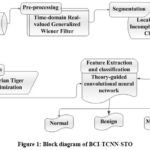Figure 1: Block diagram of BCI-TCNN-STO   Click here to view Figure

The BCI-TCNN-STO system’s block diagram is shown in Figure 1. The BCI-TCNN-STO model is used to classify images of breast cancer. Below is a full explanation of pre-processing, image segmentation, feature extraction, and classification.  The MIAS dataset is the source of the input image. The TRG-WF model is used to the picture data for the pre-processing technique. Localized Sparse Incomplete Multi-view Clustering (LSPIMC) is used to segment pre-processed images. Using a theory-guided convolutional neural network (TCNN), features of ROI images are extracted and the breast cancer images are classified. Siberian Tiger Optimization (STO) optimizes the TCNN classifier to precisely classify the breast cancer images. Accordingly, a detailed depiction of each step as follows,

Data Acquisition

The Mammographic Image Analysis Society dataset is where the input images are gathered. The MIAS in the United Kingdom provides the MIAS Database. The mammograms are digitally resized to pixels with a pixel edge of 200 microns. The ground truth for each abnormality is provided by the MIAS database as circles with approximate centres and radii for each aberration. The database contains several different kinds of abnormalities, such as calcification, masses, asymmetry, and architectural deformation. Some mammograms are deemed normal since they are devoid of any abnormalities. There are three different kinds of background tissues: dense-glandular, fatty, and fatty-glandular.

Pre-processing using Time-domain Real-valued Generalized Wiener Filter

In this section pre-processing by TRG-WF is discussed. TRG-WF acts as a pre-processor to reduce noise in images and increase the image quality. TRG-WF reduces noise without sacrificing image quality; it is suitable for many imaging applications where noise reduction is crucial. While preserving crucial image elements like boundaries and textures. The proposed TD-GWF uses a real-valued linear transform to convert a 1-D image into the 2-D image, much like the short-time Fourier transform  Luo et al.¹⁹ It is shown in equation (1)

Where, X_n,s signifies s^th frame of image form A with sample images at n^th observation, respectively. The image X_n features  are splitted and joined to create V groups of transformed images of shape X, are used to calculate a TD-GWF V_n via minimum MSE estimation. It is shown in equation (2)

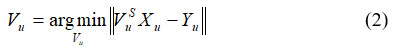
Where, Y_u indicates the error data and X_u  represents image samples. Estimation of V_u based on real-valued matrices. V_u utilized to Xˆ_u attain u^th group of output. It is shown in equation (3)

Where, Y_u denotes the set of image samples and V^s_u denotes the reduction of noise in the image. Since TD-GWF doesn’t use complex-valued operations, it avoids several possible problems with picture noise reduction and a few implementation best practices that make the system more reliable and faster during training and perform better during inference. The final output of noise reduction in the image is shown in equation (4)

Where, {Y_u}^v_{u = 1} denotes noise-reduced image samples v. By applying the training objective function to the outputs from each separation module, the system can be trained. The training procedure improves the image quality and a learnable image quality changer D € R^sxL is then applied. It is shown in equation (5)

Where, LAC(.) denotes overlap-add operation on windows and D^s Ỹ  denotes high-quality images. The input data has undergone effective preprocessing by reducing the noise and enhancing the image quality, using TRG-WF. The preprocessed data is fed into LSIMC for the image segmentation process.

Segmentation using Localized Sparse Incomplete Multi-View Clustering

This section discusses image segmentation using LSIMC Liu et al.¹⁸ The pre-processed images are segmented utilizing the LSIMC method. ROI, segmented images are categories into which the images are divided. LSIMC is a useful method for image segmentation that can help extract crucial information from complex image data. To facilitate data clustering, LSIMC focuses on extracting a structured, consistent, sparse latent representation from partial multi-view data. Accordingly, the new objective function of LSIMC is shown in equation (6)

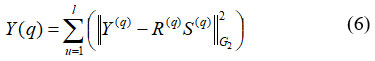
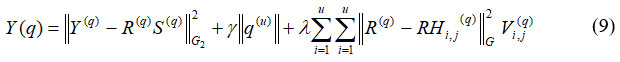
Where, Y^(q) refers to the image features to be segmented, R^(q) S^(q) refers to the image quality of features, G₂  G denotes the number of feature samples and ϖ denotes the constant variable. In segmentation, images are the information sources, and the attributes taken out of these images are the outputs. The image is divided into its main areas or components. The apparent difficulty served as the basis for the segmentation process. Four fundamental techniques are used to segment high-quality images: threshold systems, methods based on boundaries, methods combining boundary and region conditions, and hybrid procedures as shown in equation (7).

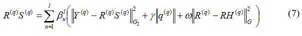
Where, γ||q^(q)|| denotes the threshold factor, β^l_u is the limit variable at q^th junction, ||R^(q) – RH^(q)|| denotes the segmented images with region, and boundary conditions. Evaluation keeps running by thresholding process as well analyzed, conventional techniques. To separate the histogram into breast tissue and background regions, as expressed in Equation (8), thresholding typically involves choosing an appropriate gray-level value based on the estimated gray-level histogram.

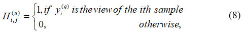
Where, H^(u)_I,j   refers to the grey-level histogram image and y_i^(q) denotes the breast tissue and background in the same order of i^th condition. An ROI is a chosen subsection of tests from the dataset that has been identified for a particular purpose. An ROI is an area of the image that needs to be filtered to carry out various actions on it. Making binary mask – binary image similar size as training image used to represent an ROI, its thresholding is shown in equation (9)

Where, H_i,j^(q) denotes the filtered ROI of the image with  i^th and j^thcondition and V_i,j^(q) refers to the binary image of ROI. Every chosen image is subjected to a segmentation procedure. The size of segmented ROI obtained from the method varies as clusters vary in size. However, segmented ROI must be picture size for uniformity, is shown in equation (10)

Where, R^(q) V^(q) H^(q) S^L refers to the segmented image size and Lr denotes the systematic view of the segmented ROI images. These images are specified as input to the TCNN model for the extraction and classification process.

Feature extraction with classification using theory-guided convolutional neural network

This section discusses the feature extraction, and classification utilizing TCNN Wang et al.²⁷ TCNN classifier extracts the ROI images. The Grayscale statistics features such as area, Diameter, Perimeter, Mean, Compactness, Variance, Entropy, Standard Deviation, Entropy, and Correlation are extracted from the segmented images. A model with convolutional layers is the TCNN. Essentially, the purpose of these layers is to recognize characteristics in the images. Every time the part of the photos is developed, TCNN learns the module of the images. Images close to structural features were extracted using each neuron in the layer. The weights of individual neurons are adjusted within the node layer to generate comparative features for the input image channel, as represented in Equation (11).

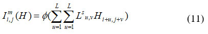
Where, L^s_u,v denotes the quantity of output layer channels, H_i+u,j+v signifies the selected features and Φ represents activation layer function at L^th location. The description of the features set can signify how the density of tissue of the breast, a challenging task for enlargement of the framework, to extract the ROI image from the features precisely. It is shown in equation (12).

Here, represents the image of the permeability field; S denotes a time matrix whose identical elements correspond to a specific time step; V indicates the image of well positions; ω refers to the TCNN parameter; and Q_V^L,S represents the precise distribution of the extracted features. For traditional CNN, the surrogate method is able to be trained by grey image mismatch among labeled grey image, forecasts, it is shown in equation (13)

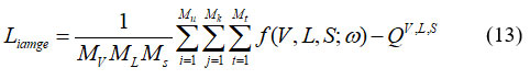
Where, M_v represents the number of well-position locations in the training dataset; M_L indicates the number of permeability layer realizations; M_s  represents the number of time phases in all realization; Q^V,L,S denotes the extracted features. Visually evaluating the images and assigning them to one of the four groups is challenging. The texture of such a region might serve as a useful tool for tissue identification in addition to structural and spectral characteristics. It signifies statistical descriptors derived from the co-occurrence matrix or the picture intensities histogram. To achieve the best depiction of breast tissue density, many feature sets are combined. Regardless, descriptors that depend on histograms lack information about a pixel’s location about another pixel. Statistics were taken from intensity levels to preserve spatial data on pixel intensity. Since well-known descriptors were employed investigation, correlation evaluates the strength of the relationship between a pixel and its neighbour as well as the degree of association. This work goes into great detail on ten different qualities. The classification is depending on data that was used to calculate attributes. A nucleus area that includes the total number of pixels could be used to characterize the nucleus zone. It is represented in equation (14)

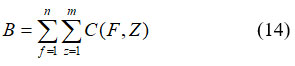
B refers nucleus zone; C signifies x as rows, y columns of segmented images. Nucleus intensity is the average pixel intensity for a certain nucleus area. Diameter is the measurement of the greatest circle’s diameter that encloses the nucleus zone. It is represented in equation (15)

Where, F₁,Z₁ and F₂,Z₂ are endpoints on the major axis. The boundary shows the length of the nucleus zone given in equation (16)

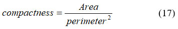
Where,  refers to the extracted features for classification and (count)unit denotes the number of feature samples noted. Compactness shows the proportion of area with a perimeter square. It is given in equation (17).

Average ROI pixel rate. It was necessary to recognize the intensity of ROI as cancer has an enormous estimation of brightness. It was expressed in equation (18).

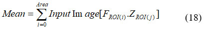
Where, F_ROI(i) denotes the extracted ROI image at i^th layer and F_ROI(j) denotes the extracted ROI image at j^th layer. Then variation is the evaluation of the distance between dual clusters. Clustering by clusters was described by random variables F, data change between dual cluster F, Z. Thus V(F, Z)  is given in equation (19).

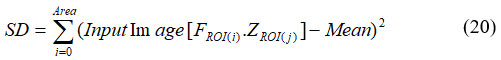
Where, H(F) was the entropy of F, (F,Z) was mutual data among F and Z. V(F, Z) estimates clusters task of objects in clustering F decrease uncertainty by object’s clusters in clustering Z. The RMS deviation of qualities from the number mean is known as the standard deviation. It was the widely recognized estimation of factual scattering, which calculated the degree to which an informative index’s attributes were distributed widely. If data points are generally near the mean, the standard deviation is close to zero. The SD is far from zero when that much data is concentrated far from the mean. When all information values are equal, the standard deviation is zero. The tumor is far from zero. It was expressed in equation (20).

An extremely disorderly appropriation is compared to a large estimate of entropy, which is defined as the assessment of disarray in object grey-level association. Low entropy images are essentially simple. A perfectly flat image has zero entropy. The minimum entropy evaluation of cancer is negative. It was expressed in equation (21).

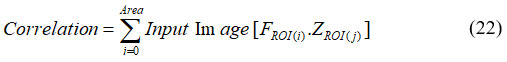
Where, NH is the normalized histogram vector. The most well-known measurable strategy is correlation. Total pixel sets for intensity levels, isolated with few separations, and few related tendencies, make up the components of the co-occurrence network. Furthermore, a relationship yields broad significance when a question includes a significant number of closely related subcomponents of constant grey level and significant grey level disparities between neighboring sections. Thus, the tumor is highly valued for this characteristic. It was expressed in equation (22).

To train a TCNN, input was sustained to the first layer, allowing the network to compute and extract features before producing the final output. After analyzing the outcome, the error was calculated and backpropagation was used to spread it in reverse throughout the network. Parameters are enhanced at each stage of the system’s development to reduce failure. This process moves forward with the data and keeps improving the system. TCNN training is an iterative, multi-layer procedure where each layer receives input and its parameters are improved until the system advances. Convolutional, fully linked, and pooling layers are the three important layers used in the construction of TCNN architecture. Most of these layers are added sequentially to create a full TCNN architecture. Following the categorization process, breast cancer images are categorized as normal, benign, or malignant. It is shown in equation (23)

Where, I_BC(w) and I_IC(w) indicates the output of the benign and malignant images, I_GE(w) shows the normal output image and I_image(w) denotes data stored in the TCNN parameter. In the final step, the loss function is minimized to compute the parameters of TCNN. TCNN method successfully extracted and classified the breast cancer images. It is classified as normal, benign, and malignant. Here, STO is employed to enhance the TCNN optimum parameter (w and S ).STO was employed for tuning the weight, and bias parameters of TCNN.

Optimization using Siberian Tiger Optimization

The STO for optimizing TCNN is discussed ³². In order to precisely classify breast cancer, the parameters of TCNN model are improved by the practice of STO. Northeast China, North Korea, Russian Far East are the home ranges of the Siberian otherwise Amur tiger, species of Panthera Tigris. Siberian tigers are incredibly swift and nimble for their size. They are formidable hunters. Siberian tigers hunt by first choosing their prey, then attacking it, and then pursuing the prey. Siberian tigers involve in contest with brown, and black bears as a result of disagreements over territory and self-defense. Siberian tiger ambushes and strikes bear from above in this fight. Then uses one forepaw to block the bear’s chin, another to grip its throat, and lastly, it bites the bear’s spine to kill it.

Step 1: Initialization

The pseudo-code for the suggested algorithm incorporates parameter changes, population evaluation, and population initialization. Equation (24) provides a mathematical representation for the steps of the proposed STO.

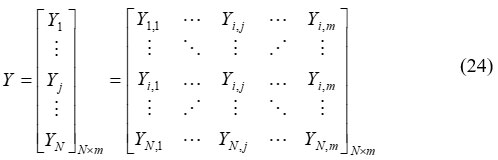
Where, Y denotes the population matrix of Siberian tigers’ positions Y, is j^th Siberian tiger, N signifies total Siberian tigers.

Step 2: Random generation

Random choices are created for the input parameters. The Optimal Progressive value is chosen according to their particular hyperparameter conditions.

Step 3: Fitness function

It uses initialized values to generate a random solution. This can be found in equation (25)

Where, ω shows the decrease in error rate and S shows the increase in accuracy

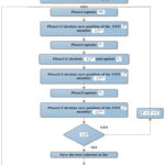Figure 2: Flowchart of STO for optimizing TCNN   Click here to view Figure

Step 4: Exploration Phase (Prey hunting)

In the initial phase, the population’s positions are adjusted according to the prey’s movement and selection behavior. This process enhances the algorithm’s global search and exploration efficiency by introducing abrupt and significant changes in the positions of the Siberian Tiger Optimization (STO) agents. Within the STO framework, each tiger determines its potential prey position from other population members that possess superior objective function values compared to its own. Equation (26) provides the set of prey locations.

In this context, Y_best represents the optimal candidate solution (the most efficient STO member), while denotes Y_k the total number of candidate solutions within the population. From this group, a specific member qq_j is randomly selected to serve as the target prey for the j^th Siberian tiger, after which its updated position is calculated. The subsequent phase focuses on refining the positions of population members through the pursuit strategy. During this stage, the Siberian tigers dynamically alter their positions within the vicinity of the prey to simulate an adaptive hunting mechanism. This strategy enhances the algorithm’s local search capability, thereby improving convergence and solution quality. To replicate the chase behavior more effectively, a new region adjacent to the current attack zone is designated for each Siberian tiger, as formulated in Equation (27).

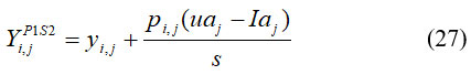
Where, Y_i,j^P1S2 denotes the new location of j^th Siberian tiger depend on the second stage of the initial phase of STO. Then, if the value of an objective function is increased, this newly calculated location replaces the previous position of the related member. It is shown in equation (28).

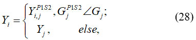
Where, G_j^P1S2 is its j^th dimension, G_j^P1S2 is its objective function value, P_i,j are random numbers in the interval [0, 1], and s is the iteration counter of the algorithm

Step 5: Exploitation Phase (Fighting with a Bear) for Optimizing and

The initial step in this phase involves the simulated attack of the j^th Siberian tiger on a bear. Other population members act as potential bears, and one bear (denoted as k) is randomly selected from this group. This interaction causes significant positional changes among the STO members, improving the algorithm’s capability to perform efficient global exploration. To model this process, a new position for each j^th STO member (j = 1,2,3,…,N ) is computed using Equation (29):

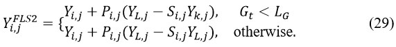
Here, Y_i,j^FLS2 denotes the j^th dimension of the bear’s position (j=1,2,3,…,n ), and is a randomly selected member from the set {1,2,…,j-1, j+1,…,N}. The term Y_i,j^FLS2represents a novel position of the j^th member during the second phase of STO, while P_i,j denotes random numbers within the range [0,1]. The parameter S_i,j serves as an optimization coefficient, as described by Aassila et al.¹

In the second stage, the positions of population members are updated by simulating conflicts during combat. This mechanism causes slight positional changes within the population, thereby improving the STO algorithm’s exploitation capability for local search. A random position near the battleground is then selected to emulate this competitive behavior. The computation is carried out using Equation (30):

where Y_i,j^FLS2 indicates the updated position of the j^th Siberian tiger during the second stage of the exploitation phase, u_θ and I_θj denote the updated and initial positions respectively, and represents the iteration counter of the algorithm.

Step 6: Termination condition

The weight bound of the generator from TCNN is enhanced by utilizing STO; it repeats step 3 until it halts the criteria Y = Y + 1 is met. Then STO optimizes the parameters of TCNN. Then TCNN classifying breast cancer images is done effectively.

Results

The investigational outcomes of the proposed method are conferred. The suggested BCI-TCNN-STO technique is used on a Python 3.8 computer with 64GB of RAM, The proposed model was implemented using TensorFlow version 2.4 on a system equipped with an Intel(R) Xeon(R) W-2155 CPU operating at 3.30–3.31 GHz. The total number of iterations corresponded to the number of batches required to complete a single epoch under various performance metrics. Furthermore, comparative analysis using multiple evaluation indicators was conducted between the proposed BCI-TCNN-STO framework and existing benchmark methods, including CBC-MI-CNN, ADBC-MMD-DCNN, and BCD-HDL. The results from this comparison substantiate the superior efficiency and robustness of the proposed system.

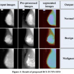Figure 3: Result of proposed BCI-TCNN-STO   Click here to view Figure

Performance measures

This is a vital phase for best classifier selection. Evaluation metrics like accuracy, F1-score, recall, precision, specificity, Error rate, and AUC are used to assess performance.

True Positive (TP): typically classifies images of breast cancer as normal;

True Negative (TN): unethically classifies images of breast cancer as normal.

False Positive (FP): often classifies the breast cancer images as either benign or malignant.

False Negative (FN): this unethical classification divides the breast cancer images into benign and malignant categories.

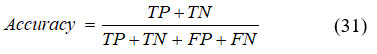
Accuracy

The accuracy of the model is defined as the ratio of correctly predicted samples to the total number of input samples, as expressed in Equation (31),

Precision

It signifies the purity of positive detections relative to ground truth computed using equation (32).

Recall

It is a metric that computes detections made by correct positive predictions created by total positive detections. It is given in equation (33),

Specificity

The model’s ability to correctly identify negative samples from the total set of actual negative instances reflects its specificity, which is mathematically represented in Equation (34).

F1- Score

The F1 score is a performance metric that integrates both precision and recall into a single harmonic mean value. It is particularly useful in scenarios where maintaining a balance between false positives and false negatives is crucial. The F1 score is mathematically defined in Equation (35).

AUC

It attains an aggregate scale of performance across each possible classification threshold, given in equation (36),

Error rate

It often signifies the frequency with which the detecting system makes inaccurate predictions or diagnoses. It is shown in equation (37)

Performance analysis

Figure 4-10 displays the simulation results of the proposed BCI-TCNN-STO approach. The CBC-MI-CNN, ADBC-MMD-DCNN, and BCD-HDL techniques are connected to the planned techniques. Table 1 shows the comparative performance of the four breast-cancer classification models (CBC-MI-CNN, ADBC-MMD-DCNN, BCD-HDL, and the performance of the proposed BCI-TCNN-STO model was assessed using multiple evaluation metrics, including Accuracy, Precision, Recall, Specificity, F1-Score, Error Rate, and Area Under the Curve (AUC).

Metric	Class	CBC-MI-CNN	ADBC-MMD-DCNN	BCD-HDL	BCI-TCNN-STO (Proposed)
Accuracy (%)	Normal	79.72	71.78	70.73	99.80
	Benign	73.71	82.69	82.74	99.30
	Malignant	70.81	79.69	79.44	99.40
Precision (%)	Normal	71.54	84.58	77.53	99.32
	Benign	74.04	84.58	77.53	99.02
	Malignant	79.14	70.81	82.65	99.27
Recall (%)	Normal	73.54	82.58	74.53	98.65
	Benign	70.74	75.61	73.95	99.04
	Malignant	74.14	71.61	73.65	98.93
Specificity (%)	Normal	76.54	70.58	82.53	99.70
	Benign	71.04	85.61	72.95	99.30
	Malignant	78.14	71.71	83.65	99.40
F1-Score (%)	Normal	77.54	69.58	72.53	98.98
	Benign	73.04	81.61	82.95	99.30
	Malignant	79.14	70.71	72.65	99.40
Error Rate (%)	Normal	27.00	17.00	15.00	0.70
	Benign	20.00	22.00	14.00	0.34
	Malignant	27.00	10.00	19.00	0.60
AUC (%)	Overall	90.87	91.76	93.56	99.34

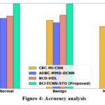Figure 4: Accuracy analysis   Click here to view Figure

Figure 4 illustrates the comparative accuracy analysis of the proposed model. The optimization strategies incorporated within the system significantly enhance classification accuracy. Consequently, the proposed BCI-TCNN-STO framework achieves 20.28%, 28.22%, and 29.27% higher accuracy for normal samples; 26.29%, 17.31%, and 17.26% higher accuracy for benign samples; and 29.19%, 20.31%, and 20.56% higher accuracy for malignant samples when compared to the existing methods, namely CBC-MI-CNN, ADBC-MMD-DCNN, and BCD-HDL, respectively.

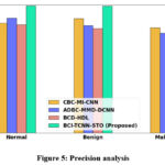Figure 5: Precision analysis   Click here to view Figure

Figure 5 presents the precision analysis of the proposed model. The incorporation of the TCNN architecture within the system contributes to a significant improvement in precision performance. As a result, the proposed BCI-TCNN-STO model achieves 28.26%, 15.22%, and 22.27% higher precision for normal samples; 25.26%, 18.59%, and 26.35% higher precision for benign samples; and 20.26%, 28.59%, and 16.75% higher precision for malignant samples when compared with the existing methods, namely CBC-MI-CNN, ADBC-MMD-DCNN, and BCD-HDL, respectively.

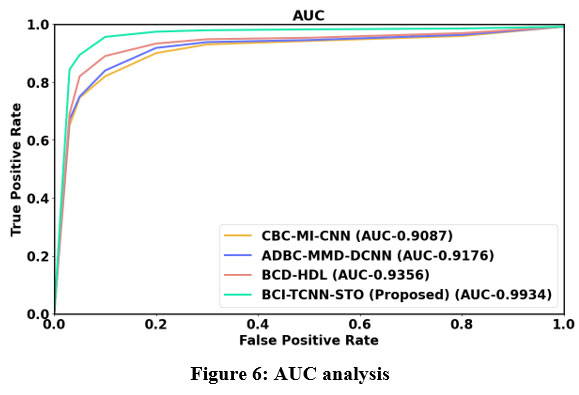Figure 6: AUC analysis     Click here to view Figure

Figure 6 shows the AUC analysis. TCNN model that is proposed in this system, leads to higher AUC. Thus, the proposed BCI-TCNN-STO model attains 25.26%, 16.22%, and 26.27% higher AUC estimated to the current technique such as CBC-MI-CNN, ADBC-MMD-DCNN and BCD-HDL, respectively.

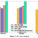Figure 7: F1- score analysis     Click here to view Figure

Figure 7 illustrates the F1-score analysis of the proposed system. The integration of the TCNN model enhances both precision and recall, resulting in a substantial improvement in the overall F1-score. Consequently, the proposed BCI-TCNN-STO framework achieves 22.26%, 30.22%, and 27.27% higher F1-scores for normal samples; 26.26%, 17.69%, and 16.35% higher for benign samples; 20.26%, 28.69%, and 19.75% higher for malignant samples; 23.66%, 17.59%, and 26.35% higher for severe DR cases; and 20.26%, 28.69%, and 19.75% higher for PDR cases compared to the existing approaches, namely CBC-MI-CNN, ADBC-MMD-DCNN, and BCD-HDL, respectively.

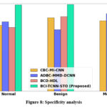Figure 8: Specificity analysis     Click here to view Figure

Figure 8 presents the specificity analysis of the proposed framework. The LMSCT-based feature extraction technique incorporated in this system significantly enhances the model’s ability to correctly identify negative instances, thereby improving specificity. As a result, the proposed BCI-TCNN-STO model achieves 23.26%, 29.22%, and 17.27% higher specificity for normal samples; 28.26%, 13.69%, and 26.35% higher for benign samples; 21.26%, 27.69%, and 15.75% higher for malignant samples; 28.26%, 13.69%, and 26.35% higher for moderate DR cases; 28.66%, 27.59%, and 16.65% higher for severe DR cases; and 21.26%, 27.69%, and 15.75% higher for PDR cases when compared with the existing models, namely CBC-MI-CNN, ADBC-MMD-DCNN, and BCD-HDL, respectively.

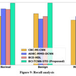Figure 9: Recall analysis     Click here to view Figure

Figure 9 shows recall analysis. The TCNN-based classification approach improves the recall of the proposed model. Thus, the proposed BCI-TCNN-STO model attains 26.26%, 17.22%, and 25.27  higher recall for normal; attains 28.56%, 23.69%, and 25.35% higher recall for benign; attains 25.26%, 27.79%, and 25.75% higher recall for malignant; attains 28.56%, 23.69%, and 25.35% higher recall for moderate DR; attains 27.66%, 28.59%, and 26.65% higher recall for severe DR; attains 25.26%, 27.79%, and 25.75% higher recall for PDR estimated to the current technique such as CBC-MI-CNN, ADBC-MMD-DCNN and BCD-HDL, respectively.

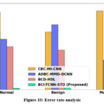Figure 10: Error rate analysis     Click here to view Figure

Figure 10 shows the error rate analysis. The BCI-TCNN-STO model attains 15.26%, 16.22%, and 18.27%  lower error rate for normal; attains 18.66%, 13.69%, 15.35% lower error rate for benign; attains 15.26%, 17.79%, 15.75% lower error rate for malignant; attain 18.66%, 13.69%, and 15.35% lower error rate for moderate DR; attain 17.66%, 19.59%, 16.65% lower error rate for severe DR: attains 15.26%, 17.79%, and 15.75% lower error rate for PDR estimated to the current technique such as CBC-MI-CNN, ADBC-MMD-DCNN and BCD-HDL, respectively.

Discussion

The proposed BCI-TCNN-STO model achieved markedly higher accuracy, specificity, and F1-scores compared with CBC-MI-CNN, ADBC-MMD-DCNN, and BCD-HDL. While these results demonstrate the technical potential of the method, several factors may have contributed to the performance beyond architectural improvements. For example, the preprocessing pipeline and parameter tuning may have enhanced feature separability, and the dataset composition—particularly the ratio of malignant to benign cases—could have favored models with higher sensitivity. Furthermore, the small error rates of the proposed approach should be interpreted with caution, as overfitting or hidden biases in the training data may partly explain the near-perfect metrics.

From a clinical perspective, a system that reliably distinguishes malignant from benign lesions could help reduce diagnostic workload and support early detection. However, real-world deployment would require validation on larger, multi-center cohorts, assessment under varying imaging conditions, and evaluation of integration into clinical workflows. Incorporating clinician feedback and prospective trials will be essential to confirm whether the observed gains translate into improved patient outcomes. Future work will also explore how the model handles edge cases, such as rare tumor subtypes, to ensure robust clinical applicability.

Conclusion

The Classification of Breast Cancer Images using Theory-guided CNN optimized with Siberian Tiger Optimization (BCI-TCNN-STO) was successfully implemented and evaluated on the MIAS dataset using a Python-based framework. The proposed method systematically explores TCNN architectures for breast cancer image feature extraction and classification, identifying the configuration that yields the strongest performance. Compared with existing techniques—CBC-MI-CNN, ADBC-MMD-DCNN, and BCD-HDL—the BCI-TCNN-STO model achieved 23.26%, 29.22%, and 17.27% higher specificity, and 22.26%, 30.22%, and 27.27% higher F1-scores, respectively. While these results demonstrate clear improvements within the experimental setting, they should be interpreted cautiously. The analysis is limited to the MIAS dataset, and factors such as dataset composition, preprocessing, and parameter tuning may have contributed to the observed gains. Future studies with larger, multi-center datasets and prospective validation are necessary to confirm the model’s robustness and to evaluate its potential clinical applicability.

Acknowledgement

The author would like to thank the Management, Principal & Head of the Department of P.S.R. Engineering College, Sivakasi for allowing us to do the research in the laboratory

Funding Sources

The author(s) received no financial support for the research, authorship, and/or publication of this article.

Conflict of Interest

The author(s) do not have any conflict of interest.

Data Availability Statement

This statement does not apply to this article.

Ethics Statement

This research did not involve human participants, animal subjects, or any material that requires ethical approval.

Informed Consent Statement

This study did not involve human participants, and therefore, informed consent was not required.

Clinical Trial Registration

This research does not involve any clinical trials.

Permission to reproduce material from other sources

Not Applicable

Author contributions

• Vinoth Rathinam: Conceptualization, Methodology, Writing – Original Draft.
• Sasireka Rajendran: Data Collection, Analysis, Writing – Review & Editing.
• Valarmathi Krishnasamy: Visualization, Supervision, Project Administration.
• Vimala Mannarsamy: Data Collection, Analysis, Writing – Review & Editing.

Reference

1. Aassila H, Aboussabiq F, Dari K, et al. Biodecolorization of Methyl Orange by bacteria isolated from textile industrial wastes: optimization of cultural and nutritional parameters. J Mater Environ Sci. 2018;9(10):2779–2787.
2. Albalawi U, Manimurugan S, Varatharajan R. Classification of breast cancer mammogram images using convolution neural network. Concurrency Comput Pract Exp. 2022;34(13):e5803.
   CrossRef
3. Aljuaid H, Alturki N, Alsubaie N, et al. Computer-aided diagnosis for breast cancer classification using deep neural networks and transfer learning. Comput Methods Programs Biomed. 2022;223:106951.
   CrossRef
4. Aly GH, Marey M, El-Sayed SA, Tolba MF. YOLO-based breast masses detection and classification in full-field digital mammograms. Comput Methods Programs Biomed. 2021;200:105823.
   CrossRef
5. Borah N, Varma PSP, Datta A, et al. Performance analysis of breast cancer classification from mammogram images using vision transformer. In: Proc IEEE CALCON.
   CrossRef
   
6. Chouhan N, Khan A, Shah JZ, et al. Deep convolutional neural network and emotional learning based breast cancer detection using digital mammography. Comput Biol Med. 2021;132:104318.
   CrossRef
7. Dang L-A, Chazard E, Poncelet E, et al. Impact of artificial intelligence in breast cancer screening with mammography. Breast Cancer. 2022;29(6):967–977.
   CrossRef
8. Darweesh MS, Adel M, Anwar A, et al. Early breast cancer diagnostics based on hierarchical machine learning classification for mammography images. Cogent Eng. 2021;8(1):1968324.
   CrossRef
9. Elmoufidi A. Deep multiple instance learning for automatic breast cancer assessment using digital mammography. IEEE Trans Instrum Meas. 2022;71:1–13.
   CrossRef
10. Gurudas V, Shaila S, Vadivel A. Breast cancer detection and classification from mammogram images using multi-model shape features. SN Comput Sci. 2022;3(5):404.
    CrossRef
11. Hamed G, Marey M, Amin SE, Tolba MF. Automated breast cancer detection and classification in full-field digital mammograms using two full and cropped detection paths approach. IEEE Access. 2021;9:116898–116913.
    CrossRef
12. Haq IU, Ali H, Wang HY, et al. Feature fusion and ensemble learning-based CNN model for mammographic image classification. J King Saud Univ Comput Inf Sci. 2022;34(6):3310–3318.
    CrossRef
13. Inan MSK, Alam FI, Hasan R. Deep integrated pipeline of segmentation guided classification of breast cancer from ultrasound images. Biomed Signal Process Control. 2022;75:103553.
    CrossRef
14. Joseph AA, Abdullahi M, Junaidu SB, et al. Improved multi-classification of breast cancer histopathological images using handcrafted features and deep neural network (dense layer). Intell Syst Appl. 2022;14:200066.
    CrossRef
15. Kanya Kumari L, Naga Jagadesh B. An adaptive teaching learning-based optimization technique for feature selection to classify mammogram medical images in breast cancer detection. Int J Syst Assur Eng Manag. 2024;15(1):35–48.
    CrossRef
16. Kaur A, Rashid M, Bashir AK, Parah SA. Detection of breast cancer masses in mammogram images with watershed segmentation and machine learning approach. In: Artificial Intelligence for Innovative Healthcare Informatics. Springer; 2022. p. 35–60.
    CrossRef
17. Khamparia A, Bharati S, Podder P, et al. Diagnosis of breast cancer based on modern mammography using hybrid transfer learning. Multidimens Syst Signal Process. 2021;32:747–765.
    CrossRef
18. Liu C, Wu Z, Wen J, et al. Localized sparse incomplete multi-view clustering. IEEE Trans Multimedia. 2022;25:5539–5551.
    CrossRef
19. Luo Y. A time-domain real-valued generalized Wiener filter for multi-channel neural separation systems. IEEE/ACM Trans Audio Speech Lang Process. 2022;30:3008–3019.
    CrossRef
20. Melekoodappattu JG, Subbian PS, Queen MF. Detection and classification of breast cancer from digital mammograms using hybrid extreme learning machine classifier. Int J Imaging Syst Technol. 2021;31(2):909–920.
    CrossRef
21. Muduli D, Dash R, Majhi B. Automated diagnosis of breast cancer using multi-modal datasets: A deep convolution neural network based approach. Biomed Signal Process Control. 2022;71:102825.
    CrossRef
22. Niu J, Li H, Zhang C, Li D. Multi‐scale attention‐based convolutional neural network for classification of breast masses in mammograms. Med Phys. 2021;48(7):3878–3892.
    CrossRef
23. Pavithra M, Rajmohan R, Kumar TA, Ramya R. Prediction and classification of breast cancer using discriminative learning models and techniques. In: Machine Vision Inspection Systems Volume 2: Machine Learning‐Based Approaches. p. 241–262.
    CrossRef
24. Raaj RS. Breast cancer detection and diagnosis using hybrid deep learning architecture. Biomed Signal Process Control. 2023;82:104558.
    CrossRef
25. Salama WM, Aly MH. Deep learning in mammography images segmentation and classification: Automated CNN approach. Alex Eng J. 2021;60(5):4701–4709.
    CrossRef
26. Singla C, Sarangi PK, Sahoo AK, Singh PK. Deep learning enhancement on mammogram images for breast cancer detection. Mater Today Proc. 2022;49:3098–3104.
    CrossRef
27. Wang N, Chang H, Zhang D, et al. Efficient well placement optimization based on theory-guided convolutional neural network. J Pet Sci Eng. 2022;208:109545.
    CrossRef
28. Zhao W, Wang R, Qi Y, et al. Bascnet: Bilateral adaptive spatial and channel attention network for breast density classification in the mammogram. Biomed Signal Process Control. 2021;70:103073.
    CrossRef