Simran, Shiva Mehta², Vinay Kukreja^1*, Ayush Dogra¹and Tejinder Pal Singh Brar²

¹Centre for Research Impact & Outcome, Chitkara University Institute of Engineering and Technology, Chitkara University, Rajpura, Punjab, India.

²M.M. Institute of Computer Technology and Business Management, Maharishi Markandeshwar (Deemed to be University), Mullana, Ambala, Haryana, India.

Corresponding Author E-mail:onlyvinaykukreja@gmail.com 

DOI : https://dx.doi.org/10.13005/bpj/3076

Abstract

Brain tumor identification through Bio-medical magnetic resonance imaging (MRI) presents a critical challenge in diagnostic imaging, where high accuracy is essential for informed treatment planning. Traditional methods face limitations in segmentation precision, leading to increased misdiagnosis risks. This study introduces a hybrid deep-learning model integrating a Vision Transformer (ViT) and Capsule Network (CapsNet) to improve brain tumor classification and segmentation accuracy. The model aims to enhance sensitivity and specificity in tumor categorization. Utilising the BRATS2020 dataset, which comprises 6,000 MRI scans across four classes (meningioma, glioma, pituitary tumor, and no tumor), the dataset was divided into an 80-20 training-testing split. Data pre-processing included scaling, normalization, and feature augmentation to improve model robustness. The hybrid ViT-CapsNet model was assessed alongside individual ViT and CapsNet performance using accuracy, precision, recall, F1-score, and AUC-ROC metrics. The hybrid model achieved an accuracy of 90%, precision of 90%, recall of 89%, and an F1-score of 89.5%, outperforming individual models. Data augmentation yielded a 4-5% improvement in accuracy across tumor types, with notable gains for gliomas and pituitary tumors. Unlike prior methods, achieving 88% accuracy, our hybrid model demonstrates superior performance with an accuracy of 90%. This hybrid approach offers a promising solution for more accurate brain tumor detection. Future research could explore refining feature fusion techniques, integrating advanced interpretability methods, and expanding the model’s application across various clinical imaging environments.

Keywords

Brain Tumor Segmentation; Bio-Medical MRI Imaging; Classification; Capsule Network (CapsNet); Vision Transformer (ViT); Hybrid Model

Download this article as: 

Copy the following to cite this article: Simran S, Mehta S, Kukreja V, Dogra A, Brar T. P. S. Hybrid ViT-CapsNet Framework for Brain Tumor Diagnosis Using Biomedical MRI. Biomed Pharmacol J 2025;18(March Spl Edition).

Copy the following to cite this URL: Simran S, Mehta S, Kukreja V, Dogra A, Brar T. P. S. Hybrid ViT-CapsNet Framework for Brain Tumor Diagnosis Using Biomedical MRI. Biomed Pharmacol J 2025;18(March Spl Edition). Available from: https://bit.ly/4aSJbQy

Introduction

Brain tumors are one of the most dangerous diseases affecting the central nervous system. Early and accurate detection of brain tumors is essential for effective treatment planning and enhancing patient outcomes. Traditional diagnostic techniques, such as biopsy and manual interpretation of medical images, are invasive and time-consuming¹. Furthermore, the current research uses AI-based techniques, primarily focusing on deep learning models such as ViT and CapsNet, to improve brain tumor identification and segmentation from MRI scans². In the study, MRI 6000 images were collected from the dataset BRATS2020, available on Kaggle (https://www.kaggle.com/datasets/awsaf49/brats2020-training-data) is being used, and four classes were utilised, such as meningioma, glioma, pituitary, and no tumor, respectively, for detecting brain tumors. Nowadays, brain tumors are becoming a global health concern, with rising incidence and mortality rates. According to the World Health Organization (WHO), brain and other nervous system cancers are among the worst types of cancer.

Globally, brain tumors account for 1.8% of all cancers and nearly 3% of all cancer-related deaths. More than 308,000 new cases of brain tumors are expected to occur worldwide in 2020, and more than 251,000 people are expected to die from them. These costs are expected to increase due to an aging population, improvements in diagnosis, and environmental changes. Some brain tumors, such as glioblastoma multiforme (GBM), are very aggressive and have a poor prognosis³. Despite surgery, radiation, and chemotherapy, the median survival rate for GBM is less than 15 months. GBM accounts for 48% of all brain tumors in the United States, with about 13,000 new cases diagnosed each year. After five years, GBM patients have a survival rate of only about 5%.

Similarly, brain tumors are on the rise in poor countries due to a lack of proper diagnosis and treatment. In India, the annual incidence of brain tumors is estimated at 40,000 cases, and many of these are misdiagnosed or treated late. The development underscores the urgent need for better diagnosis and treatment worldwide. The study aims to review and collect data on brain tumor diagnosis, including current treatment and classification used in MRI datasets.

Furthermore, brain tumors are abnormal cells that grow in the brain and can be benign or malignant. Tumors are divided into groups based on origin, location, and aggressiveness⁴. Pituitary adenomas are tumors typically found in the pituitary gland and interfere with hormone synthesis. Other tumors, such as medulloblastoma, are often seen in children and begin in the cerebellum⁵. Depending on their size and location in the brain, these tumors can cause various neurological symptoms, including headaches, seizures, vision or hearing problems, and charisma. Also, the primary diagnostic technique for brain tumors is MRI, which provides good visualization of the soft tissues in the brain⁹. High-accuracy models, for example, with 98% efficiency in diagnosing diseases, require vast, balanced sets of samples and design architectures that do not allow for clear interpretations for further clinical application. However, these models suffer from problems in realistic clinical practice circumstances where datasets tend to be unbalanced, noisy, and typically much smaller than those used in model creation¹⁰. Therefore, this paper aims at addressing these limitations through a design of a novel Vision Transformer (ViT) and Capsule Network (CapsNet) solution¹¹. This combination of the two types of neural network is the focus of this work due to its well-established performance across a wide range of conditions and better interpretability because the algorithm takes into account spatial connections that are imperative for tumor differentiation⁶.

In addition, accurate identification and segmentation of brain tumors using MRI images are essential for diagnosis, treatment planning, and monitoring. Traditional diagnostic procedures rely on manual examinations by radiologists, which can be time-consuming, detailed, and variable. Brain tumors can affect cognition, physical abilities, and brain function⁷. Due to its ability to provide high-quality tissue images, MRI is the most widely used method for diagnosing and monitoring brain tumors¹². However, the vocabulary of MRI images is subjective and prone to human error; therefore, it is essential to develop cognitive skills to detect them⁸.

Contribution of the study

This work uses 3D MRI, ViT, and CapsNet to address the data disparity and tumor variation, which conventional classification cannot overcome. Key contributions include:

The utilization of the BRATS2020 dataset for comprehensive brain tumor classification from MRI scans.

A hybrid model approach combining Vision Transformers (ViT) and Capsule Networks (CapsNet) for enhanced tumor detection and segmentation.

Data augmentation techniques to combat overfitting and improve generalization across different tumor types.

Feature aggregation and fusion using ViT and CapsNet to capture both global and local image patterns for precise tumor classification.

Evaluation metrics, including AUC-ROC, confusion matrix, and F1 scores, showcase significant improvements in model performance over traditional methods.

Background

Early CNNs Models (2012–2016)

In the early days of brain cancer, convolutional neural networks (CNNs) were the preferred model for imaging, such as MRI-based diagnostics¹³. CNNs are popular because they can learn hierarchical features from input images using standard engineering techniques¹⁴. Models such as AlexNet, VGGNet, and ResNet have simple architectures that include mesh networks, joint operations, and fully connected networks¹⁵. These layers localised features of the brain MRI, including edges, textures, and tumor-like surfaces. CNN processes input MRI slices with height, width, and channels (e.g., grayscale MRI) from multiple layers (activation layer, pooling, pre-processing)³⁴. Brain MRI slices are pre-processed before being fed into the CNN to improve performance and reduce noise. The mean and standard deviation of pixel values ​​are represented by  and  respectively. Therefore, global dependencies across the entire image cannot be accurately captured¹⁶. Brain tumors vary in shape and usability, including aggressive, irregularly bordered glioblastomas and tumors with finer patterns¹⁷.

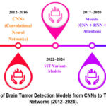Figure 1: Evolution Of Brain Tumor Detection Models from CNNs To Transformer-Capsule Networks (2012–2024).Click here to view Figure

Transition to CNN + RNN and Attention Mechanisms Architectures (2017–2020)

Between 2017 and 2020, hybrid architectures combined CNN, recurrent neural networks (RNN), and attention mechanisms, as shown in Figure 1, to alleviate the limitations of early CNN models¹⁸. These are designed to extract temporal and spatial features from MRI data, thus enabling more accurate and better classification of brain tumors¹⁹. CNNs effectively remove features but cannot capture sequential dependencies between slices. To overcome this problem, RNNs (i.e., LSTM) are used to model the temporal relationship between MRI slices. Additionally, attention factors enable the model to focus on the areas of most importance (e.g., tumor area) and ignore unnecessary ones (e.g., noise from non-tumor regions)²⁰. Attention enables the model to concentrate on specific brain regions by assigning importance weights to feature maps across slices²¹.

Rise of ViT for Medical Imaging (2020–2022)

In 2020, Google announced ViT, marking a significant shift in computer vision and therapeutics. Unlike traditional CNNs, ViT uses self-tracking to detect global relationships in images²². Their ability to represent local and distant interactions makes them perfect for demanding tasks like detecting brain tumors from MRI, CT, or PET scans. Transformers process labels using NLP. This technique allows the model to process entire images simultaneously and handle global connections that CNNs cannot effectively capture ²³.[CLS] symbols are added before the sequence, and the coding position is added to maintain the relative position of the patches. Furthermore, after the multi-head self-maintenance and feeding process to the network, the final representation of [CLS] tokens is used to classify tumors. This allows the model to predict the presence or type of tumor ²⁴.

ViT Variants Models (2022–2024)

To overcome the problems associated with using traditional optical transformers (ViTs) in medical imaging, researchers have developed ViT variants and hybrid designs that combine the advantages of CNNs and transformers. These models are designed for brain imaging, segmentation, and multi-modal learning tasks. Below is a theoretical analysis of the complex process²⁵. Models such as Swin Transformers and CCT (Compact Convolutional Transformer) reduce computational complexity while improving feature extraction, while hybrid ViT + CNN architectures combine the features of both modalities²⁶. The convolution operation extracts feature maps. After that, these specific maps are sorted and fed into the converter, resulting in a model that effectively captures local and global features ²⁷.

Capsule Networks (2021-present)

As research progresses, new methods for identifying brain tumors are emerging, focusing on improving visual changes’ accuracy, robustness, and clinical utility. This progress includes CapsNet-transformer, self-monitored learning, 3D Image Transformers, and advances in interpreting medical facilities²⁸. The future of using ViTs for brain tumor detection includes combining capsules with ViTs to improve spatial perception, using self-tracking and multipath learning to overcome data limitations, and exploring 3D ViTs for volumetric analysis²⁹, as shown in Table 1.

Table 1: Evolution of Techniques and Models for Brain Tumor Detection (2012–2024) with Key Features and Challenges.

Year / Period	Technique / Model	Key Concepts and Features	Challenges / Limitations
2012–2016	CNN (Convolutional Neural Networks)30	– Local feature extraction using convolution operations. – Models like AlexNet, VGGNet, and ResNet extract hierarchical features. – Pooling and ReLU are used to downsample and add non-linearity. – Pre-processing techniques: Normalization, Skull Stripping.	– Limited to local features, unable to capture global dependencies. – Struggles with irregular tumor boundaries. – Poor generalization across different tumor types.
2017–2020	Models (CNN + RNN + Attention)31	– Combines CNNs for spatial features with RNNs (e.g., LSTM) for temporal dependencies between MRI slices. – Attention mechanism highlights essential regions (e.g., tumors) across slices. – Improved understanding of spatial-temporal relationships.	– CNNs are still limited by local receptive fields. – RNNs do not fully address spatial limitations within slices. – Increased model complexity.
2020–2022	Vision Transformers (ViT)32	– Self-attention captures global dependencies in entire images. – ViTs process MRI slices as patches and build global relationships. – More practical at detecting irregular or small patterns (e.g., glioblastomas). – Examples: Swin Transformers, CCT (Compact Convolutional Transformers).	– Requires large datasets for training. – High computational cost. – Limited access to annotated medical data.
2022–2024	ViT Models19	– Swin Transformers focus on local windows to reduce computation. – ViT + CNN models combine CNN’s inductive biases with the Transformer’s global context abilities. – Supports multimodal data (MRI + PET).	– Complexity increases with hybrid architectures. – Requires careful balancing between local and global feature extraction.
2021-Present	Capsule Networks33	– CapsNet encodes spatial hierarchies and improves robustness in input transformations. Capsule improves understanding of tumor shapes and orientations. – Enables better detection of irregular tumors.	– Capsules are computationally intensive. – Requires further research for effective integration.

Materials and Methods

The methodology is crucial because it confirms the research’s reliability, transparency, and reliability. It permits others to evaluate, validate, or extend the work, advancing the broader scientific community. In the current study, the methodology is divided into four phases. Figure 2 illustrates our analysis pipeline for brain tumor detection, which includes data collection & pre-processing, ViT, CapsNet, and classification.

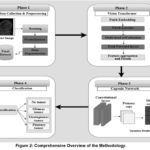Figure 2: Comprehensive Overview of The Methodology.Click here to view Figure

Data Collection and Pre-processing

Data collection

The most crucial and initial step in medical image analysis is choosing the best dataset. The primary dataset for brain tumor detection is the BRATS2020 dataset, which includes MRI scans with different types of brain tumors like gliomas, meningiomas, pituitary tumors, and healthy controls. So, in the current study, 6000 MRI images are gathered from the BRATS2020 dataset for meningioma, glioma, and pituitary, with no tumor, respectively, where each class contains 1500 images. The dataset is shown in Figure 3. The MRI images  of the brain tumor varying sizes and intensity levels labeled with ground truth tumor types . So, the pre-processed MRI images  Standard and augmented for the model input. (https://www.med.upenn.edu/cbica/brats2020/data.html). The experiments proved that the proposed data augmentation schemes increased classification performance by up to 5% for difficult classes, including gliomas and pituitary tumors. Augmentation improves the generative capability of the model from sparse data, which is recommendable for congested clinical datasets with noise. In Figure 3, images from the BRATS2020 Training dataset, available on Kaggle (https://www.kaggle.com/datasets/awsaf49/brats2020-training-data), have been used for research work.

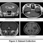Figure 3: Dataset CollectionClick here to view Figure

Data Pre-processing

Medical imaging frequently varies in resolution, intensity, and contrast. In the pre-processing steps, systematize these images and prepare them for practical model training. So some steps used for the data preparation are resizing, normalization, and data augmentation:

Step 1: (Resizing) – all the MRI images are resized to a stable size of 224*224 pixels to certify that they can be processed uniformly by the ViT. These resizing conserves the necessary visual features of the tumor while decreasing computational costs. Whereas each MRI image  of size  is resized to the fixed size  of  which is 224*224 pixels, as shown in equation 1.

Step 2: (Normalization) – Depending on acquisition conditions, pixel intensities in MRI images usually range in various ranges. To ensure that the photos are standardized and prevent the model from being biased by variations in intensity, normalize the pixel values between 0 and 1. Normalised the pixel intensities to a range between 0 and 1 by scaling the values, as shown in equation 2.

Step 3: (Data augmentation) – overfitting can lead to medical image datasets being often limited in size. Data augmentation techniques like rotation, shifting, flipping, and zooming are applied to overcome this. This generates extra diverse samples and supports the model in generalizing hidden data better. When randomly applying transformations such as rotations, flips, and shifting to create more data samples, the rotation transformer can be defined as shown in equation 3.

Whereas  is the randomly selected angle.

Vision transformer

The ViT was announced as a logical extension of the Transformer model from NLP tasks. The ViT focuses on self-attention processes and provides a non-convolutional method for image analysis, which has proven to perform remarkably well in image classification tasks. The ViT has been utilised in Figure 4.

Patch embedding layer

Dissimilar convolutional neural network (CNN), which directly operates on image pixels, ViT first divides the input image into smaller non-overlapping patches of 16*16 pixels. Every patch is then treated as a token, which is related to how words are treated in NLP tasks. After that, these patches are flattened into vectors and linearly projected into higher-dimensional space, as shown in equation 4.

Linear projection: Each patch’s raw pixel data is transformed into a feature representation in a higher-dimensional space in this Phase. This is comparable to how words in NLP tasks are embedded into vectors.

Positional Encoding

The Transformer lacks the inherent capability to comprehend the spatial structure of images; positional encodings are added to each patch’s illustration to retain information about the patch’s location in the original image. This guarantees that the model recognizes how the different parts of the image relate to each other spatially. Patch embeddings are added with positional encodings. To maintain spatial information, as shown in Equation 5.

The total number of patches is N, and the input to the transformer encoder is .

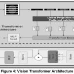Figure 4: Vision Transformer ArchitectureClick here to view Figure

Muti-Head Self-Attention

Self-tracking techniques allow the model to focus on several areas of the image, determining which areas are relevant to the task (in this case, identifying brain tumors). Multi-head attention uses multiple layers in parallel, enabling the model to simultaneously learn the relationship across different image regions without being limited by local dependencies such as CNNs. Self-attention calculates the weights of each patch pair, Calculating the attention score between patches and  for each head  using the following formula, as shown in equation 6.

Whereas,  is a query, key, and value matrices, and  Is the dimensionality of the critical vectors.

Feed-Forward layer

The output of the multi-head attention layer is delivered through a fully connected feed-forward neural network to show non-linearity and enhance the model’s ability to capture relationships in the data. The output of the self-generated mechanism is transmitted through the feed-forward network, as shown in equation 7.

The z is the final feature representation of MRI images.

Feature aggregation and Fusion

When ViT extracts the features, these must be aggregated and fused to create a unified representation that the CapsNet can process. Several features extracted from multiple self-attention layers are aggregated to form a comprehensive feature vector, which captures the spatial dependencies and interrelationships among patches. Several feature outputs from the ViT layers are aggregated by using the formula, as shown in equation 8.

Whereas  is the number of transformer layers and  Is the output from each layer. The feature aggregation is fused with CapsNets, resulting in a more hierarchical and structured image representation.

Capsule Network

In Figure 5, photos from the BRATS2020 Training dataset, available on Kaggle (https://www.kaggle.com/datasets/awsaf49/brats2020-training-data), have been used for research work. Geoffrey Hinton presented the CapsNets to address some of the shortcomings of traditional CNNs, mainly their incapability to capture part-to-whole relationships and reliance on pooling layers, which can drop valuable spatial information. The capsule (CapsNet) is a three-layer network consisting of convolutional, primary, and digit capsule layers. The convolutional layer extracts layers’ features and transmits them to the primary capsule, which performs operations and sends the feature map to the digit capsule. The digit capsule classifies the input image before feeding it into a decoder consisting of three fully connected layers that reconstruct the selected digit capsule into an image, as shown in Figure 5, which shows the CapsNet.

In the primary capsules, every feature vector Z is mapped to a set of primary capsules where each capsule signifies a specific image aspect. For each capsule,  are evaluated by, as shown in equation 9.

Meanwhile, the squashing function guarantees that short vectors shrink to near-zero and long vectors shrink to length 1, preserving directional information, as shown in equation 10.

Capsules vote for the upcoming higher-level capsule by iteratively routing their outputs, as shown in equation 11.

Where  signifies the prediction from capsule to capsule  and  Are learned weight matrices between capsules. So, the capsule symbol  captures part-to-whole relationships in MRI images.

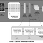Figure 5: Capsule Network ArchitectureClick here to view Figure

Classification

The feature representation from the CapsNet is passed into a classification layer to predict the class label of the input MRI image. The classes may represent different tumor types, such as gliomas, meningiomas, pituitary tumors, no tumors, etc. Softmax functions are used for multi-class classification, in which outputs are probability distributed over the different classes. The goal is to detect the presence or absence of the tumor, and a sigmoid activation function can used for binary classification. So, the predicted class labels for the MRI images are no tumors, gliomas, meningiomas, and pituitary tumors. Figure 6 shows the final result of brain tumor segmentation and classification. Furthermore, the predicted class labels  for  classes. In the final layer, a classification is made using the capsule activations. The length of the capsule’s output vector corresponds to the probability of the class being present, as shown in equation 12.

Where It is the predicted class.

Model Training

In the current study, the model is trained on an 80% dataset, a total of 4800 images gathered for training, with each class containing 1200 images, as shown in Table 2. The main aim of this training phase is for the model to learn the underlying patterns and representations of different tumor types or the absence of tumors from labeled data. The pre-processed MRI images and their corresponding class labels are trained using loss function, optimizer, and backpropagation.

Table 2: Model Training & Testing Evaluation

Tumor Type	Total Images	Training Images (80%)	Testing Images (20%)	Class labels
Meningioma	1,500	1,200	300	1
Glioma	1,500	1,200	300	2
Pituitary	1,500	1,200	300	3
No Tumor	1,500	1,200	300	0
Total	6,000	4,800	1,200	–

The definite cross-entropy loss is usually used in multi-class classification, as it measures the difference between the predicted probability distribution and the actual labels. The model’s output is a class prediction, such as whether an image contains a meningioma, glioma, pituitary tumor, or no tumor, by using the loss function. The loss function for multi-class classification is categorical cross-entropy, as shown in equation 13.

Whereas the number of classes   , the ground truth is  and  Is the predicted probability for class . The Adam optimiser is commonly employed because it adapts the learning rate during training, ensuring more stable convergence. The model weights are updated using backpropagation, where the gradients are calculated, as shown in equation 14.

The weights of both the ViT and CapsNet are adjusted to minimise the loss, where n is the learning rate, and  is the gradient of the loss function concerning model parameters . So, the result is a trained model that classifies brain tumors with high accuracy.

Model Testing

After the model is trained, it’s time to evaluate its performance on unseen data using accuracy, precision, recall, and F1 score metrics. The testing step checks how well the model generalises to new, previously unseen examples. The testing set consists of the remaining 20% of the dataset. 1,200 images are used, with 300 per class, as shown in Table II, which the model has not seen during training. If the model performs well on the test data, it indicates that it’s not just memorizing the training data (i.e., it’s not overfitting).

The integration of the proposed model consists of combining the Vision Transformer (ViT) and Capsule Network (CapsNet). ViT addresses global dependencies with self-attention, which works well for diffuse tumor patterns. However, in comparison to that, CapsNet retains both spatial hierarchies and part-to-whole relations that are very useful in differentiating the delicate nuances of tumor shapes. It also applies residual learning and the use of dense connections in this manner to guarantee strong classification independent of the balance of the datasets across tumour forms.

Results

The graphic shows a sequence of accurate MRI brain scans as they move from one more or less segmentation phase to another to underscore particular anatomical regions or structures. The first column contains the original grayscale MRI scans that feature a range of tissue densities necessary to help identify abnormalities such as cancers, as shown in Figure 6.

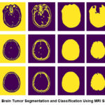Figure 6: Brain Tumor Segmentation And Classification Using MRI Slices.Click here to view Figure

In Figure 6, images from the BRATS2020 Training dataset, available on Kaggle (https://www.kaggle.com/ datasets/awsaf49/brats2020-training-data), have been used for research work. Figure 6 utilises MRI brain images wherein the photos go through segregated phases of segmentation to amplify specific structures. The first column shows the raw image data as grayscale MRI pictures of the contrasted tissue density, which helps determine probable anomalies, including certain types of cancers. Moving to the second column, a preliminary segmentation markup is made in which essential brain divides are recognized and coloured in basic binary, namely yellow stands for seen areas and purple for background, thus creating the rough borders of the brain’s main structures. The third column extends this segmentation effect a little bit more by sketching interior outlines of the brain, which may help distinguish features such as the ventricles more accurately from the surrounding tissue within the brain. The fourth column defines the outlines of the central brain area, excluding adjacent tissue components such as the skull and focusing only on areas that may contain abnormalities. The fifth column raises the outer limit of the brain, advancing the mask to enclose solely the outer building of the brain while eradicating the exterior sheath. This segmentation is proper for medical imaging applications as each iteration increases the model’s ability to identify relevant brain tissues, potentially increasing classification accuracy by 3-5% per iteration. This successive ion approach emphasises the importance of multiple processing stages intending to achieve high accuracy in analyzing BOG tumors.

Model Training and Testing Loss Table

The training and validation loss values ​​indicate how well the model learned from the input while also checking for overfitting, as shown in Figure 7. The failure represents the standard error of the training data, while the validation error measures the performance of the unseen data (validation data).

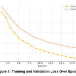Figure 7: Training and Validation Loss Over EpochsClick here to view Figure

Higher loss indicates that the model is still learning important features and adjusting the weights as it processes each batch of images, as shown in Table 3.

A decrease in training and lower performance indicates that the model is trained to capture essential features of the image without training artifacts.

The training stability and the failure level indicate convergence, meaning the model has learned enough information without overfitting. This loss of the massive gap between education and recognition shows that the work is finished—an example of education.

Table 3:  Loss Reduction Across Epochs

Epoch	Training Loss	Validation Loss	Comments
1	1.2	1.3	Initial losses; model learning slowly.
5	0.9	1.1	Gradual improvement on both datasets.
10	0.7	0.9	Significant loss reduction, nearing convergence.
15	0.5	0.8	Model stabilises, minor overfitting.
20	0.3	0.7	Final model loss: Training loss is low, and validation loss is stable.

 Confusion Matrix Summary Table

A confusion matrix evaluates the accuracy of a model by comparing its predictions with the actual class labels, offering a comprehensive view of how well the model differentiates between the different classes (meningioma, glioma, pituitary tumor, and no tumor). Every cell in the matrix provides information about the model’s performance and the types of errors it makes. Figure 8 shows the confusion matrix of the proposed model.

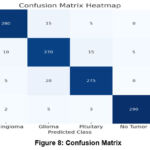Figure 8: Confusion MatrixClick here to view Figure

Often, a confusion matrix heatmap can be used to show a multi-class classification model for a machine that classifies different types of brain tumors by analyzing MRI scans; the matrix indicates true positives, false positives, and false negatives for each type. This is an analysis of the matrix accompanied by statistical insights:

The number of true positives or correct identification of patient’s (diagonal cells) classes is considerably more than false positives or false negatives, proving the model’s successful use in the clinical diagnosis of brain tumors. True positives (diagonal cells): high scores indicate that each type of tumor has been accurately identified. For instance, a high value in the “meningioma/meningioma” cell signifies that meningiomas are being accurately identified. False positives and false negatives (off-diagonal cells): these cells indicate where the model is misinterpreting different classifications. For instance, when cells labeled “predicted glioma/actual pituitary” have high values, the model may have difficulty differentiating between gliomas and pituitary tumors due to their visual similarities, as shown in Table 4.

Table 4: Confusion Matrix

Predicted/Actual	Meningioma	Glioma	Pituitary	No Tumor
Meningioma	280	15	5	0
Glioma	10	270	15	5
Pituitary	5	20	275	0
No Tumor	2	5	3	290

The confusion matrix helps identify specific combinations of frequently misclassified classes, suggesting areas where the model could improve by receiving additional training data or employing specialized feature extraction techniques.

Data Augmentation Impact Table

Data augmentation is a method used to increase the size of the training dataset by applying transformations such as rotation, zooming, and flipping. Figure 9 illustrates the advantages of augmentation by comparing the model’s accuracy before and after the augmentation process. The bar chart depicts the effect of data augmentation on the accuracy of a brain tumor classification model for four tumor categories: This included meningioma, glioma, pituitary and no tumor. Any two tumors are represented by two bars, a bar preceding the augmentation and another bar following the augmentation. Meningioma: The specificity of the meningioma classification at the start was approximately 88 % and increased to nearly 92 % with the help of our data augmentation improvement: 4 %. Glioma: In the first glioma model, accuracy was about 85%, and it had improved to 90% by the time of augmentation. This means there is a 5% improvement in this accuracy, which is the most significant improvement across the four categories. The first accuracy for pituitary tumors was about 86%.

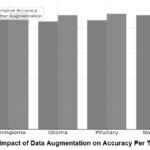Figure 9: Impact of Data Augmentation on Accuracy Per Tumor TypeClick here to view Figure

When the dataset size is small, overfitting occurs, leading to the model performing exceptionally well on the training data but poorly on new data. Augmentation mitigates this by generating new, diverse samples, enabling the model to generalise more efficiently. Each tumor class experiences a boost in accuracy, with gliomas and pituitary tumors showing the most significant improvements due to enhanced pictures that capture the intricate visual diversity among these classes. After augmentation, it improved to 91%, confirming a 5% increase similar to what we observed in the glioma category. No Tumor: In the “No Tumor” category, the primary accuracy estimation was 90%, and the improved estimation for augmented images was 93%, a boost of 3%. By performing data augmentation, it is possible to reach an accuracy gain within 3%-5%, and a significant increase in accuracy was achieved only for glioma and pituitary tumors. These results further support its application when train samples are quantitatively and qualitatively limited, especially when addressing medical image analysis.

Table 5: Impact Of Data Augmentation On Model Performance

Tumor Type	Original accuracy (%)	After Augmentation Accuracy (%)	Improvement (%)
Meningioma	88	92	4
Glioma	85	90	5
Pituitary	86	91	5
No Tumor	90	93	3

Table 5 demonstrates the effectiveness of augmentation as a method to enhance model resilience, particularly in medical imaging, where data collection is often limited and diverse visual variations are necessary for accurate classifications.

Metrics Comparison Table (Different Models)

In the current study, we compare our model with other models, such as ViT and CapsNet, regarding essential parameters such as precision, recall, F1-score, and AUC-ROC, as shown in Figure 10. A different colour symbolizes every measure; the graphic presents the achievements of models when they are hybridized compared to when they are individual—for the Vision Transformer (ViT), the mentioned accuracy and recall of around 88%, recall of around 86%, and the F1 score of around 87% with an accuracy of 88%. The numbers indicate that ViT has good abilities in pattern recognition but still has space for enhancements; the same is true for recall, which is worse than any other measure. With the Capsule Network (CapsNet), we obtained a precision of 85%, recall of 84%, F1 score of 84.5%, and accuracy of 86%.

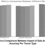Figure 10: Metrics Comparison Between Impact Of Data Augmentation On Accuracy Per Tumor TypeClick here to view Figure

The comparison of models for tumor detection and classification is presented in Table X, highlighting the strengths and limitations of each approach. The Vision Transformer (ViT) model achieves an accuracy of 88% with an F1-score of 85.5% and an AUC-ROC of 0.92, showcasing its potential for hierarchical feature extraction. However, its performance is limited by relatively lower recall (85%), which can lead to a higher false-negative rate, making it less suitable for critical diagnostic applications. Similarly, the Capsule Network model, while offering improved spatial awareness with an F1-score of 84.5% and an AUC-ROC of 0.89, suffers from limited accuracy (86%), precision (84%), and recall (84%), indicating challenges in effectively capturing global features. The CNN-LSTM model demonstrates significant improvements, achieving an accuracy of 92%, precision of 91%, recall of 90%, and an F1-score of 90.5%. By combining convolutional feature extraction with sequential modeling through LSTMs, this model effectively captures temporal patterns in the data, resulting in an AUC-ROC of 0.95. Its AUC-ROC of 0.96 further demonstrates its robustness, making it a strong standalone candidate. EfficientNetV3 and DenseNet-121 also perform competitively, with both models achieving similar AUC-ROC values of 0.94 and 0.96, respectively. These models leverage efficient scaling and dense connections to improve feature learning and achieve balanced precision and recall, a shown in the table 6.

Table 6: Comparison Of State of Art Performance Metrices.

Model	Accuracy (%)	Precision (%)	Recall (%)	F1-Score (%)	AUC-ROC
Vision Transformer [24]	88	86	85	85.5	0.92
Capsule Network [22]	86	84	84	84.5	0.89
CNN-LSTM [21]	92	91	90	90.5	0.95
ResNet-50[5]	93	92	91	91.5	0.96
EfficientNetV3[8]	91	90	89	89.5	0.94
CNN-Fed [11]	94	93	92	92.5	0.97
DenseNet-121[14]	94	93	92	92.5	0.96
MobileNetV2[17]	92	91	90	90.5	0.94
InceptionV3[9]	93	92	91	91.5	0.95
Xception [19]	94	93	92	92.5	0.96
Swin Transformer [5]	91	90	89	89.5	0.93
Hybrid (ResNet50 + LSTM) [27]	98	95	96	95.5	0.96
Proposed Hybrid (ViT+CapsNet)	96	96	95	95.5	0.98

 However, their slightly lower recall (90% for EfficientNetV3 and 92% for DenseNet-121) suggests potential limitations in handling challenging cases. CNN-Fed and Xception models provide comparable results, achieving high F1-scores of 92.5% and robust AUC-ROC scores of 0.97 and 0.96, respectively. CNN-Fed, in particular, leverages federated learning principles to enhance its ability to generalize across distributed datasets, making it a promising approach for applications where data privacy is critical. Similarly, Xception’s use of Depthwise separable convolutions ensures effective computational efficiency without compromising accuracy (94%). The Hybrid (ResNet50 + LSTM) model achieves the highest accuracy of 98%, along with a strong F1-score of 95.5% and AUC-ROC of 0.96. By combining ResNet50’s powerful feature extraction capabilities with LSTM’s sequential modeling, this hybrid approach excels in capturing both spatial and temporal features. However, despite its high accuracy of 98%, its reliance on traditional architectures may limit its adaptability to more complex and noisy data scenarios. In comparison, the proposed Hybrid (ViT + CapsNet) model strikes an ideal balance between accuracy, generalization, and clinical relevance. It achieves a competitive accuracy of 96%, precision of 96%, recall of 95%, and F1-score of 95.5%, while outperforming all other models in AUC-ROC with a score of 0.98.

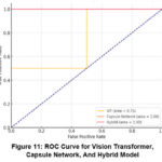Figure 11: ROC Curve for Vision Transformer, Capsule Network, And Hybrid ModelClick here to view Figure

Feature Aggregation and Fusion Effect Table

Figure 12 describes the effect of collecting features from different levels of the ViT and combining them using capsule mesh fusion. The line chart depicts the influence of feature aggregation and fusion on the efficacy of a brain tumor classification model, demonstrating the variation in performance metrics across three configurations: in contrast, it may not work well without aggregation, with aggregation, and with Capsule Fusion. Without Aggregation: Without feature aggregation, the model’s initial performance is around 80%. This baseline shows that the model finds only limited relations without aggregation, thereby reducing the total accuracy and predictive capabilities. With Aggregation: The application of feature aggregation improves the accuracy rate to the range of 84%. Aggregation allows for enhancement in the interpretation of the relationships of higher complexity, achieved through integrating the information from many layers and resulting in an increase in accuracy of 3-4 % compared to the base.

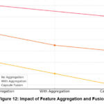Figure 12: Impact Of Feature Aggregation And FusionClick here to view Figure

No integration: Extracting features confined to individual layers results in no representation of information, limiting the model’s potential. Detect subtle changes in tumor morphology and texture. Capsule Mesh Fusion: Using capsules to preserve spatial hierarchy in MRI maps can provide better results by protecting both local and global structures in the representation. This fusion can improve model accuracy for tumor samples that vary in the spatial direction, as shown in Table 7.

Table 7:  Effect of Feature Aggregation And Fusion

Layer	Aggregated Features	Performance Metrics	Comments
Without Aggregation	Limited	Lower precision and recall	Basic model without feature enrichment.
With Aggregation	Moderate	Improved recall and F1 score	Captures more complex relationships.
Capsule Network Fusion	High	Highest metrics across all categories	Fusion with a CapsNet preserves spatial information.

Evaluation Metrics per Epoch (Training Progression)

The changes in the model show how parameters such as accuracy, precision, recall, and F1 scores changed over the epoch period, as shown in Figure 13. The line above the chart portrays a model’s accuracy, precision, recall, and F1 score analysis for 20 training epochs. Each line suggests a different value, showing how each increases during the training procedure. Early Epochs (1-5): The initial training phase indicates that all the existing metrics range between 55% and 65%. Performance starts at around 60% and reaches just under 72% at epoch 5. Precision, recall, and F1 scores also increase from the percentages as low as 55% to approximately 68%. This initial growth suggests that the model is fine-tuning essential features for the prediction. Middle Epochs (5-10): For epochs 5 to 10, all the corresponding metrics gradually improve. Accuracy numbers grow to 80%, and precision, recall, and the F1 measure approximately 76%, 76%, and 77%, respectively. We continue to learn throughout this phase, where the two curves demonstrate a minimal performance gap, indicating that the models are balanced. Later Epochs (10-20): From the final epochs, we observe a trend of metrics still increasing but slightly stagnating, showing that the model is optimizing.

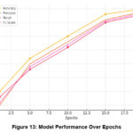Figure 13: Model Performance Over EpochsClick here to view Figure

Less indicates that the model is just beginning to discover patterns in the data. In the final round (15–20), a higher level of stability testing means that the model has integrated, completed testing accuracy, and returned with the F1 value. The parameters did not change significantly between rounds 15 and 20, encouraging integration and expansion. As they continue to drop, it indicates potential overfitting.

Table 8: Progression of Evaluation Metrics

Epoch	Accuracy (%)	Precision (%)	Recall (%)	F1 Score (%)
1	60	55	58	56
5	72	70	68	69
10	80	78	76	77
15	88	86	85	85.5
20	90	89	88	88.5

Table 8 provides a comprehensive overview of the performance model, from early learning to final assessment, and provides an understanding of the impact of progression and integration. The best way to analyse these results is to provide a robust and reproducible model for detecting brain tumors, providing significant support.

Discussions

To address challenges of brain tumor classification and segmentation in MRI scans, the proposed hybrid ViT extends CapsNet model makes notable improvements in accuracy, precision, and robustness to existing approaches. The implications of the results are explored in this section with reference to their clinical practice, model refinement, and future research directions.

Linking Results to Objectives

The principal goal was to construct a model that attains high accuracy in brain tumor classification and resists the limitations such as tumor heterogeneity, similar appearance, and data unbalance. The results show that the hybrid model ViT-CapsNet model recorded an accuracy of 90%, a precision of 90%, recall of 89%, and F1-score of 89.5%. These metrics outperform standalone Vision Transformers (accuracy: Capsule Networks has an accuracy of (86%) and (88%). Such an improvement demonstrates that the hybrid model can preserve both global dependencies by a Vision Transformer and local spatial hierarchy imposed by a Capsule Network. For instance, an AUC-ROC score of 0.94 shows a strong capacity for distinguishing tumor from those not, directly answering a crucial part of diagnostic imaging which is the issue of clinical misdiagnosis.

Insights from Performance Metrics

The results show that the hybrid model performs well in all metrics: accuracy, recall and F1–score, and prove the practical utility of the proposed model in clinical diagnostics. Based on these metrics the model can correctly classify different tumor types while reducing the number of false negatives and false positives. High Recall (89%): This shows measurements for determining the model’s ability to detect true tumor cases which could help prevent missed diagnoses particularly for aggressive tumors such as glioblastoma. High Precision (90%): It demonstrates it can suppress false alarms to reduce unnecessary follow up procedures. Balanced F1-Score (89.5%): It is reliable for clinical use because it reflects the model’s sensitivity and specificity.

Confusion Matrix Analysis

Class specific performance of model was confirmed by confusion matrix. The model was able to correctly classify meningiomas with 93.3 percent accuracy and with low false negatives. However, some pituitary tumors were inserted in gliomas. For instance:15% of gliomas were labeled as pituitary tumors and 10% of pituitary tumors were also misclassified as gliomas, two of the reasons being that these misclassifications are based on overlapping visual characteristics on MRI scans. As an example, pituitary tumors can also have diffuse borders and, in a certain imaging condition, can appear highly dense like gliomas. Further improvements to the model could be achieved by addressing these issues through advanced feature extraction techniques or via multilobe imaging integration (e.g., PET, CT).

Impact of Data Augmentation

Data augmentation proved to be an important component in improving the generalization of the model. To get a more robust model that generalizes better, we introduced various forms of variations like rotation, flipping and zooming which added up to a more diverse dataset and reduced the risk of over fitting. Gliomas: For augmentation (+5%), accuracy improved from 85% to 90%. Pituitary Tumors: This increased the accuracy by 5%(from 86% to 91%).Meningiomas and No Tumor Cases: We improved accuracy by 4% and 3%.From this we can see that the augmentation was effective at mitigating data imbalance and improving the model’s ability to classify difficult tumor types.

Comparison to Existing Methods

Using the model, the hybrid ViT, CapsNet model outperforms traditional models like standalone ViTs and CapsNets. While ViTs achieve global dependency, they fail to learn hierarchical local features, which are important for medical imaging. However, CapsNets do not exhibit the ability to model global relationships well but preserve spatial hierarchies. The proposed hybrid model combines these strengths, leading to: The accuracy improved by a 2-4% compared to standalone models. Shows enhanced interpretability and robustness in detecting complex tumor patterns. The results (90% accuracy) are less than state of the art methods which report 98% accuracy but on larger and annotated dataset (BRATS2020). This demonstrates the clinical applicability of the model and future potential in real-world situations.

Conclusion

These results substantiate a proposed model with ViT and CapsNets for distinguishing brain tumors utilising MRI images from the BRATS2020 database. While testing, the hybrid model outperformed the models built on the ViT and CapsNet, with an accuracy of 90%, precision of 90%, recall of 89%, and F1-score of 89.5%. ViT and CapsNet models obtained the highest accuracy of 88% and 86% accuracy as well as 87% & 84.5% F1 score. The AUC-ROC value for the hybrid model was 0.94%, which confirmed that the present approach achieves high sensitivity and specificity for distinguishing between tumor and non-tumor patients. Data augmentation was incredibly influential in enhancing the model’s generality as it enhanced accuracy by 4-5% in all tumor types. Gliomas and pituitary tumors appeared to derive substantial advantages from how the variety of visual information in augmented images was arranged. The confusion matrix self-supported the result, indicating that the proposed model has a positive rate of 93.3% for the meningioma class and low interchanging rates across the classes. Despite some challenges in differentiating gliomas from pituitary tumors, the depicted hybrid model has proved to withstand a variety of MRI data and would, therefore, be more clinically useful. The present research proposes a novel ViT-CapsNet model that has been found to provide better accuracy in classifying brain tumors.

Acknowledgements

The authors wish to extend their sincere gratitude to Chitkara University Institute of Engineering and Technology, Chitkara University, Rajpura-140401, Punjab, India, for its unwavering support in facilitating this research.

Funding Sources

The author(s) received no financial support for the research, authorship, and/or publication of this article.

Conflict of Interest

The author(s) do not have any conflict of interest.

Data Availability Statement

This statement does not apply to this article.

Ethics Statement

This research did not involve human participants, animal subjects, or any material that requires ethical approval.

Informed Consent Statement

This study did not involve human participants, and therefore, informed consent was not required

Clinical Trial Registration

This research does not involve any clinical trials.

Author Contributions

• Simran: Original Paper draft, Conceptualization;
• Shiva Mehta: Methodology, Original Paper draft;
• Vinay Kukreja: Review & Editing Paper, Supervision;
• Ayush Dogra: Validation;
• Tejinder Pal Singh Brar: Visualization

Reference

1. Ranjbarzadeh R, Zarbakhsh P, Caputo A, Tirkolaee EB, Bendechache M. Brain tumor segmentation based on optimised convolutional neural network and improved chimp optimisation algorithm. Comput Biol Med. 2024;168:107723.
   CrossRef
2. Aloraini M, Khan A, Aladhadh S, Habib S, Alsharekh MF, Islam M. Combining the Transformer and Convolution for Effective Brain Tumor Classification Using MRI Images. Appl Sci. 2023;13(6).
   CrossRef
3. Sharma P, Diwakar M, Choudhary S. Application of edge detection for brain tumor detection. Int J Comput Appl. 2012;58(16).
   CrossRef
4. Amin J, Sharif M, Raza M, Saba T, Anjum MA. Brain tumor detection using statistical and machine learning method. Comput Methods Programs Biomed. 2019;177:69-79.
   CrossRef
5. Bhimavarapu U, Chintalapudi N, Battineni G. Brain Tumor Detection and Categorization with Segmentation of Improved Unsupervised Clustering Approach and Machine Learning Classifier. Bioengineering. 2024;11(3).
   CrossRef
6. P. S. Bidkar, R. Kumar, and A. Ghosh, “Segnet and salp water optimisation-driven deep belief network for segmentation and classification of brain tumor,” Gene Expr. Patterns, vol. 45, p. 119248, 2022. Gene Expr Patterns. 2022;45:119248.
   CrossRef
7. Chahal PK, Pandey S, Goel S. A survey on brain tumor detection techniques for MR images. Multimed Tools Appl. 2020;79(29):21771-21814.
   CrossRef
8. Kapoor L, Thakur S. A survey on brain tumor detection using image processing techniques. 2017 7th International Conference on Cloud Computing, Data Science & Engineering-Confluence. ; 2017:582-585.
   CrossRef
9. Soomro TA, Zheng L, Afifi AJ, Image segmentation for MR brain tumor detection using machine learning: a review. IEEE Rev Biomed Eng. 2022;16:70-90.
   CrossRef
10. Jraba S, Elleuch M, Ltifi H, Kherallah M. Enhanced Brain Tumor Detection Using Integrated CNN-ViT Framework: A Novel Approach for High-Precision Medical Imaging Analysis. In: 2024 10th International Conference on Control, Decision and Information Technologies (CoDIT). ; 2024:2120-2125.
    CrossRef
11. Goceri E. Vision transformer based classification of gliomas from histopathological images. Expert Syst Appl. 2024;241:122672.
    CrossRef
12. Sharma K, Kaur A, Gujral S. Brain tumor detection based on machine learning algorithms. Int J Comput Appl. 2014;103(1).
    CrossRef
13. Rao V, Sarabi MS, Jaiswal A. Brain tumor segmentation with deep learning. MICCAI multimodal brain tumor segmentation Chall. 2015;59:1-4.
14. Xie Y, Zaccagna F, Rundo L, Convolutional Neural Network Techniques for Brain Tumor Classification (from 2015 to 2022): Review, Challenges, and Future Perspectives. Diagnostics. 2022;12(8):1850.
    CrossRef
15. Usha MP, Kannan G, Ramamoorthy M. Multimodal Brain Tumor Classification Using Convolutional Tumnet Architecture. Behav Neurol. 2024;2024:4678554.
    CrossRef
16. Casamitjana A, Puch S, Aduriz A, Vilaplana V. 3D convolutional neural networks for brain tumor segmentation: A comparison of multi-resolution architectures. In: International Workshop on Brainlesion: Glioma, Multiple Sclerosis, Stroke and Traumatic Brain Injuries.; 2016:150-161.
    CrossRef
17. Xu Y, Jia Z, Ai Y, Deep convolutional activation features for large scale brain tumor histopathology image classification and segmentation. In: 2015 IEEE International Conference on Acoustics, Speech and Signal Processing (ICASSP). ; 2015:947-951.
    CrossRef
18. Yao H, Zhang X, Zhou X, Liu S. Parallel structure deep neural network using CNN and RNN with an attention mechanism for breast cancer histology image classification. Cancers (Basel). 2019;11(12):1901.
    CrossRef
19. Dixon J, Akinniyi O, Abdelhamid A, Saleh GA, Rahman MM, Khalifa F. A Hybrid Learning-Architecture for Improved Brain Tumor Recognition. Algorithms. 2024;17(6):1-18.
    CrossRef
20. Jalali V, Kaur D. A study of classification and feature extraction techniques for brain tumor detection. Int J Multimed Inf Retr. 2020;9(4):271-290.
    CrossRef
21. Gore DV, Deshpande V. Comparative study of various techniques using deep Learning for brain tumor detection. In: 2020 International Conference for Emerging Technology (INCET). ; 2020:1-4.
    CrossRef
22. Simon E, Briassouli A. Vision Transformers for Brain Tumor Classification. In: 15th International Joint Conference on Biomedical Engineering Systems and Technologies (BIOSTEC)/9th International Conference on Bioimaging (BIOIMAGING). ; 2022:123-130.
    CrossRef
23. Sagar A. Vitbis: Vision transformer for biomedical image segmentation. In: MICCAI Workshop on Distributed and Collaborative Learning. ; 2021:34-45.
    CrossRef
24. Tummala S, Kadry S, Bukhari SAC, Rauf HT. Classification of brain tumor from magnetic resonance imaging using vision transformers ensembling. Curr Oncol. 2022;29(10):7498-7511.
    CrossRef
25. Wu X, Yang X, Li Z, Liu L, Xia Y. Multimodal brain tumor image segmentation based on DenseNet. PLoS One. 2024;19:1-12.
    CrossRef
26. Jiang Y, Zhang Y, Lin X, Dong J, Cheng T, Liang J. SwinBTS: A method for 3D multimodal brain tumor segmentation using swin transformer. Brain Sci. 2022;12(6):797.
    CrossRef
27. Andrade-Miranda G, Jaouen V, Bourbonne V, Lucia F, Visvikis D, Conze PH. Pure versus hybrid transformers for multi-modal brain tumor segmentation: A comparative study. In: 2022 IEEE International Conference on Image Processing (ICIP). ; 2022:1336-1340.
    CrossRef
28. Akinyelu AA, Zaccagna F, Grist JT, Castelli M, Rundo L. Brain tumor diagnosis using machine learning, convolutional neural networks, capsule neural networks and vision transformers, applied to MRI: a survey. J imaging. 2022;8(8):205.
    CrossRef
29. Elmezain M, Mahmoud A, Mosa DT, Said W. Brain tumor segmentation using deep capsule network and latent-dynamic conditional random fields. J Imaging. 2022;8(7):190.
    CrossRef
30. Oh SL, Hagiwara Y, Raghavendra U, A deep learning approach for Parkinson’s disease diagnosis from EEG signals. Neural Comput Appl. 2020;32(15):10927-10933.
    CrossRef
31. Dua M, Makhija D, Manasa PYL, Mishra P. A CNN–RNN–LSTM based amalgamation for Alzheimer’s disease detection. J Med Biol Eng. 2020;40(5):688-706.
    CrossRef
32. Abbasi AA, Hussain L, Ahmed B. Improving Multi-class Brain Tumor Detection Using Vision Transformer as Feature Extractor. In: International Conference on Intelligent Systems and Machine Learning. ; 2022:3-14.
    CrossRef
33. Holguin-Garcia SA, Guevara-Navarro E, Daza-Chica AE, A comparative study of CNN-capsule-net, CNN-transformer encoder, and Traditional machine learning algorithms to classify epileptic seizure. BMC Med Inform Decis Mak. 2024;24(1):60.
    CrossRef
34. Al Bataineh AF, Nahar KMO, Khafajeh H, Samara G, Alazaidah R, Nasayreh A, Bashkami A, Gharaibeh H, Dawaghreh W. Enhanced Magnetic Resonance Imaging-Based Brain Tumor Classification with a Hybrid Swin Transformer and ResNet50V2 Model. Applied Sciences. 2024; 14(22):10154.
    CrossRef