Swapna Katta¹, Prabhishek Singh^2*, Deepak Garg¹and Manoj Diwakar³

¹School of Computer Science and Artificial Intelligence, SR University, Warangal, Telangana, India

²School of Computer Science Engineering and Technology, Bennett University, Greater Noida, India

³Department of CSE, Graphic Era Deemed to be University, Dehradun, Uttarakhand, India.

Corresponding Author E-mail:prabhisheksingh1988@gmail.com

DOI : https://dx.doi.org/10.13005/bpj/3078

Abstract

This paper introduces a new deep learning paradigm using the Denoising Convolutional-Neural Network (DnCNN) model for denoising Gaussian noise in Computed Tomography (CT) images. By nature, Gaussian noise is inherently random and additive, potentially obscuring vital diagnostic features and significantly reducing image quality, resulting difficulties in medical interpretation. Initially, the distorted images are sourced from addition of Gaussian noise with different intensity levels (σ = 5,10,15,20). The denoising process of DnCNN model employs a deep convolutional neural network that maps the noisy image to clean image, focusing on residual learning to prevent loss of detail. The CT images obtained after denoising are assessed using quantitative measures like Peak signal to noise ratio (PSNR), Signal to noise ratio (SNR), Structural similarity index measure (SSIM) and Entropy difference (ED). The proposed DnCNN model is evaluated using quantitative metrics, such as PSNR, SNR, SSIM, and ED, demonstrating better performance than standard denoising algorithms, including Total Variation, BM3D, Guided, Bilateral, and Anisotropic Diffusion filters. The experimental results show that the proposed DnCNN model outperforms conventional methods. The model achieves a PSNR of 35.66 dB, an SNR of 30.16 dB, SSIM of 0.91 and ED of 0.35. Additionally, zooming analysis and intensity profile evaluations confirms that the proposed method effectively suppresses noise while preserving sharper edges and finer anatomical structures. This ensures superior visual quality and greater efficacy compared to traditional methods. These experimental findings confirm that the proposed method is a robust denoising strategy in medical imaging for predicting accurate diagnostic outcomes.

Keywords

CT image; Deep learning; Denoising; DnCNN; Gaussian noise

Download this article as: 

Copy the following to cite this article: Katta S, Singh P, Garg D, Diwakar M. An Efficient Gaussian Noise Denoising in CT Images with Deep Convolutional Neural Networks. Biomed Pharmacol J 2025;18(March Spl Edition).

Copy the following to cite this URL: Katta S, Singh P, Garg D, Diwakar M. An Efficient Gaussian Noise Denoising in CT Images with Deep Convolutional Neural Networks. Biomed Pharmacol J 2025;18(March Spl Edition). Available from: https://bit.ly/4bmrSYn

Introduction

CT imaging is a diagnostic imaging technology used to acquire cross-sectional images of radiation-sensitive organs. However, the radiation risks associated with X-rays have raise concerns about cancer. To address this, Low dose CT (LDCT) minimizes radiation exposure by diminishing X-ray flux, which can notably impact the image quality acquired from sensors. The minimization of radiation dose inherently increases noise and potentially compromises diagnostic precision.¹ LDCT images are normally associated with greater noise and artifacts than images produced using normal dose CT, which influences imaging quality. LDCT medical images are often contaminated by various kinds of noise such as Gaussian and salt-and-pepper noise. Gaussian blur noise caused by electronic interference, as well as image processing, reconstruction, and quantization, affects image quality. Gaussian noise is caused by random changes in pixel values, resulting pixel blurring and weakened image sharpness and fine detail preservation.^2,3 Hence, denoising LDCT images is crucial to obtain clear image for better disease diagnosis.

The major objective of denoising CT images is to suppress noise while preserving structural information like textures, edges, and artifact suppression. The major categories of CT image denoising methods comprise of conventional methods, deep learning approaches, and hybrid approaches.^4-6 Conventional methods such as mean, Gaussian, bilateral, nonlocal mean filters, Block matching 3D filtering (BM3D) and wavelet based denoising, perform noise suppression. The Discrete Wavelet Transform (DWT) is also used for noise suppression and fine detail preservation, but choosing the right wavelet basis and thresholding method is important for achieving a balance between noise elimination and fine detail retention. However, conventional filtering methods struggle to preserve fine details in images, face difficulties in managing intricate noise patterns, requires parameter tuning, and generate artifacts, which limit their efficacy in medical diagnosis.

Consequently, recent advancements in deep learning technology contribute a powerful substitute, leveraging large datasets to train superior noise reduction patterns, such as Convolutional Neural Networks (CNNs) for denoising LDCT images.⁷ CNNs can extract features from raw inputs, reducing the need to manually select features from the dataset. They detect complex image patterns and handle different kinds of noise, making them suitable for denoising. CNNs improve processing speed and throughput with their end-to-end learning methodology. They preserve fine image details and can be easily scaled and adjusted to different applications and datasets. CNNs are preferably used in image processing applications such as refinement and denoising. A CNN consists of several convolutional layers, pooling layers and fully-connected layers. The CNN layer uses kernels to capture image features by utilizing raw data and also suppresses noise effectively. However, when dealing with shallow networks, might be insufficient to adequately learn and capture inherent complexity of very deeper networks. Residual encoder-decoder CNN (RED-CNN) and UNet framework overcome the challenge of training deeper networks and solving the vanishing gradient problem. RED-CNN effectively focusing on learning the residuals between noisy and clean images, thereby the network improves denoising effectiveness.⁸ However, the resulting image is overly smooth and has some areas in the image are locally distorted. U-Net, originally intended for medical image segmentation, exhibits impressive performance in denoising CT images as a result of its encoder-decoder model is accompanied by skip-connections, which maintain the spatial relationship between image features.⁹ These methods are very effective because they can give a global context of the images which gives superior results in minimizing noise.

LDCT image reconstruction enhancement has greatly improved with the utilization of Generative Adversarial Networks (GANs) to minimize distortion effects. However, issues such as instability in training and mode collapse and slow convergence have led researchers to constantly work on optimizing GAN architectures and algorithms. A variant of GANs, like WGAN (Wasserstein GAN), suppress noise while maintaining image details and also avoid vanishing gradient problems. Deep learning-based neural networks can suffer from the vanishing gradient problem when the gradients of the loss function become minuscule as they are backpropagated through the layers of the deep neural network, making it difficult for the network to learn features effectively. WGAN employs the use of Wasserstein distance to represent distribution loss and perceptual loss. While traditional GANs use Jensen-Shannon divergence, WGAN uses earth-mover’s distance, which provides smoother gradients. An enhanced GAN combines various loss functions, such as perceptual loss, adversarial loss and structural-similarity loss, to improve training stability and speed.¹⁰ CycleGAN is a kind of GAN developed for unsupervised image-to-image translation tasks.¹¹ It improves the training stability, convergence and resolves problems relating to vanishing gradients in deeper networks. However, these methods predominantly aim at extracting features and modifying the network structure using convolutional layers to detect only local-regions, making it difficult to capture the global context.

To overcome these issues, Transformer models, such as Vision Transformer (ViT), work well for denoising CT images. ViT leverages the self-attention mechanism to recognize long-range contextual relationships and global dependencies across the whole image, which is particularly useful in MRI scans. However, ViT faces computational bottlenecks since it requires full-image attention.¹² In the case of ultrasound imaging, where images are significantly affected by speckle noise, Transformers have demonstrated improved performance in handling noise owing to their capability to learn various patterns of noise. Various enhancements have been made to the vision transformer to enhance local feature learning and suppress computational overhead. These include local and mixed attention models, which have led to the development of Pyramid Vision Transformer and Uformer. However, these models often overlook local details, and the image after noise-mitigation can still interfere clinical diagnostic assessments. Compared to CNN architectures, Transformers generally perform better in recognizing long-range dependencies recognition but require more computational time. Denoising autoencoders (DAEs) are another deep learning technique for denoising tasks. The major disadvantage of DAEs is that they are computationally lightweight architectures. However, they lack the ability to capture global patterns like the Transformers. Nevertheless, Transformers outperform CNNs in tasks involving complex noise reduction. At the same time, CNNs are efficient, work better in extracting local features, and remain a relevant choice in terms of efficiency.

Hybrid methods play a crucial role in CT image denoising. These methods combine traditional approaches with deep learning techniques to leverage the advantages of both. For instance, hybrid methods may use a CNN as a pre-processing step for noise removal, followed by a conventional algorithm for further enhancement. A new and improved hybrid architecture called Swin-Conv-UNet (SCUNet) is proposed to minimize interference in X-ray fluorescence computed tomography (XFCT) images, particularly at low tracer concentrations. The model, trained using augmented data, utilizes deep learning frameworks to optimize image quality, achieving 39.05 PSNR and 0.86 SSIM compared to traditional and advanced methods such as BM3D, BM4D, and DnCNN. This approach is one of the primary methods for enhancing XFCT imaging while minimizing radiation exposure.¹³

Major contributions

This paper explores a DnCNN-based model which is employed for the suppression of Gaussian noise in CT images while maintaining relevant diagnostic features. The deep learning model is capable of rapidly adapt to complex noise patterns derived from the information extracted during the image processing, considerably improving the overall imaging quality. Medical imaging applications provide a scalable solution for noise suppression effectively. Deep learning-based denoising guarantees a secure and impactful method for noise suppression, contributing to the development of accurate clinical diagnoses.

Literature review 

Medical imaging approaches are categorized based on the imaging modality used, the type of image produced, and their relevance to diagnosis or investigation. These techniques include X-ray, CT scan, magnetic resonance imaging (MRI), ultrasound, and positron emission tomography (PET).³ The most effective denoising methods vary across modalities due to differences in spatial detail, temporal-resolution, cost, and the characteristics of each scanning technique. Spatial and temporal resolution are two essential aspects that characterize medical image quality and the performance of denoising algorithms. High spatial resolution can increase noise levels, and high temporal resolution can cause motion artifacts. Spatial and temporal resolution are especially important for LDCT and dynamic CT images, as well as clinical studies, involving spatial and temporal analysis. Several deep learning techniques, such as CNNs, Transformers, and CNN with Recurrent Neural Network (RNN) integrated models, have been investigated to address these problems. These approaches have exhibited superior results in effectively suppressing noise while maintaining fine image features. Spatial resolution is crucial in imaging as it makes it helps to distinguish small structures in images. In lung cancer screening using LDCT, high spatial resolution is critical for early-stage detection of small pulmonary nodules, while low spatial resolution causes blurriness, complicating early detection. Temporal resolution, essential for dynamic imaging, plays a vital role in coronary CT angiography, especially in visualizing the beating heart and coronary arteries. High temporal resolution reduces motion artifacts that interfere with diagnosis, while transformer-CNN architectures improve the images by minimizing noise as well as capturing temporal dependencies across frames.

Each medical imaging modality introduces various types of noise, requiring tailored approaches for optimal noise suppression. CT scans use X-rays to generate sliced grayscale images of the human body, characterizing tissue densities. In LDCT images, reduced radiation increases noise due to fewer X-ray photons being detected by the scanner, resulting in lower signal strength and higher noise levels. The increased noise compromises image quality, making it more difficult to detect subtle features. The lower radiation levels, while limiting patient exposure, result in both Gaussian and Poisson noise in CT images. Gaussian noise arises from electronic imperfections or noise during the image reconstruction process, while Poisson noise occurs due to the statistical randomness of photons detected by the CT scanner. These types of noise degrade image quality and diagnostic proficiency. CT image denoising methods are required to suppress the noise, there by producing cleaner images to improve diagnostic accuracy.

Denoising can be achieved using traditional methods, iterative reconstruction methods and deep learning-based methods. Traditional methods include spatial and frequency domain filters.¹⁴ Spatial filters manipulate the image pixels, such as Gaussian, median, mean filter and bilateral filters, while frequency domain filters transform the image into frequency domain using Fourier transform. Examples of frequency domain filters include anisotropic diffusion, wiener filter and nonlocal means filter. These traditional denoising methods effectively suppress noise but can also blur fine details of CT images. Advanced noise suppression methods, such as iterative reconstruction (IR) and deep learning-based approaches, are employed to enhance overall image quality in LDCT images. Iterative reconstruction methods pass through multiple iterations to refine the image by comparing actual measured data with estimated projectional data. The IR method effectively minimizes noise and artifact intensity while preserving the significant image features, leading to better resolution in LDCT images. However, the iterative reconstruction process heavily depends on iterative calculations and the quality of input image data and mathematical models, making it computationally intensive.

Recently, deep learning has played a significant influence on image denoising within contemporary science. In LDCT images, deep learning-based methods such as CNNs, GANs, and autoencoders have shown considerable improvements in image quality compared to conventional techniques. Deep learning-based denoising methods like CNNs can learn mappings between distorted and clean CT images, while GANs generate realistic denoised CT images using a generator and discriminator. Autoencoders are able to compress and reconstruct image data to mitigate noise, whereas Transformer models capture long-range dependencies and contextual data for enhanced noise suppression. These enhanced methods offer high-quality noise suppression to improve overall imaging quality.

The novel approach for medical image denoising, consists of a deep CNN, adaptive watershed segmentation, and a hybrid lifting scheme, is applied based on modified bi-histogram equalization, as suggested by Annavarapu.¹⁵ The CNN effectively minimizes noise while preserving image details necessary for diagnostic analysis. Adaptive watershed Segmentation enhances the recovery of minute details in the image, increasing the probability of extracting detailed information from other parts of the image. The hybrid lifting scheme improves contrast, making it easier to distinguish the important features. Marker-based watershed segmentation further reduces the occurrence of information loss during denoising. The proposed approach achieves a Jaccard index of 0.95, demonstrating a high segmentation accuracy. Additionally, it obtains a PSNR of 43.76 dB, highlighting the efficacy of the methodology in denoising medical images. However, the method may struggle with high-frequency noise, potentially resulting in information loss. Its complexity could hinder scalability and practical implementation. Furthermore, reliance on specific metrics may not fully reflect its effectiveness across diverse medical imaging scenarios.

A novel hybrid loss function combining MSE with a Pearson-based metric to enhance texture preservation in LDCT image denoising was introduced by Oh et al.¹⁶ Experimental results show that, significant improvements in texture quality over traditional MSE and GAN methods, maintaining a balance between noise suppression and detail retention. A robust hybrid loss-based network (RHLNet) advances LDCT image quality, supporting more accurate clinical diagnoses and marking a valuable contribution to medical imaging, as proposed by Saidulu et al.¹⁷ The RHLNet is effectively utilized in LDCT denoising, employing both shallow and deep structures, along with lattice residual blocks, to maintain image details. Shallow structures represent the initial layers of the RHLNet and extract low-level features such as edges and textures, while deep structures extract high-level and complex patterns by progressively combining and refining the basic features obtained from the shallow layers. The lattice residual block in RHLNet enhances feature representation and improves model’s learning efficiency. The RHLNet provides better performance in preserving textures due to the introduction of the Huber loss and also maintains the desired suppression capability from the Charbonnier loss. The Charbonnier loss is generally applied in image restoration tasks, like denoising, to manage outliers and enhance noise minimization.

The performance of the model is further strengthened by optimizing VGG19 on the NIH-AAPM-Mayo Clinic low dose CT (LDCT) Grand challenge dataset, ensuring that important image details are retained. Performance assessments on the large-volume dataset prove the RHLNet’s effectiveness with significant enhancements of LDCT images. However, the methodology could have issues with computation and a severe dependence on data quality for model training. The main challenges to implement RHLNet are high computational cost and handling high resolution and noisy data, leading to low generalization and low texture production in images with high or noisy backgrounds.

The low and high-frequency alignment (LHFA) model, which addresses domain shift challenges related to DL-based low-dose CT image denoising by aligning low and high-frequency attributes across various datasets, was suggested by Huang et al.¹⁸ It integrates a Low-frequency Alignment (LFA) module to preserve crucial semantic information and a High-frequency Alignment (HFA) module that recognizes noise discrepancies in latent space by applying an autoencoder. The integration of the LFA and HFA modules can be implemented in either a sequential or parallel way. In the sequential approach, LFA initially captures global features (smoother features, overall anatomical structures), followed by HFA to refine high-frequency details (edges and textures). This method improves performance. However, it could result in increased latency. Conversely, the parallel method allows LFA and HFA modules to independently process low and high frequency components, subsequently fusing their outputs for final image reconstruction. Both methods effectively mitigate noise while preserving image details, with the sequential approach emphasizing refinement and the parallel approach optimizing computational efficiency. The model proficiently maintains diagnostic image quality with noise suppression and demonstrates strong cross-domain adaptability and performance for new medical image applications through transfer learning and fine-tuning modules, although it necessitates extensive computational power due to its high-level alignment modules. The performance of the model can be improved through lightweight networks and two additional optimization methods called pruning and quantization as well as hardware acceleration through GPUs and TPUs.

A generic framework is specifically implemented for denoising LDCT-acquired images, which adopts deep neural networks with an attention mechanism to refine feature extraction and facilitate multi-scale fusion, was implemented by Niknejad Mazandarani et al.¹⁹ The model incorporates a new type of residual block focusing on feature learning and presents a structural loss to retain structural components and high-frequency (edge) details. The findings from the experiments confirms, significant enhancements in image quality in LDCT images, precisely mitigating noise that diminishes diagnostic accuracy.

An Adaptive noise aware denoising Generative-Adversarial-Networks (ANAD GAN), which make use of a cognitive noise-memory module intended to decode contextual features varying with noise level and automatically recalibrate feature vectors was introduced by Jin et al.²⁰ The noise-memory module trained using a self-updating mechanism to dynamically refine feature vectors based on noise intensity levels, improving robustness and maintaining fine image details compared to conventional methods. Moreover, the framework combines an application-specific block, termed as BLOGS, to improve the interpretations of noise distributions and applies a detail-preserving discriminator-based loss-function to fine-tune image details. The BLOGS block is designed to enhance noise distribution interpretation by adaptively extracting multi-scale noise features and refining them using hierarchical attention mechanisms. This approach depicts a strong capability to operate flexibly at different noise levels, reaching the optimal results with PSNR > 50.74 and SSIM > 0.99 across range of datasets. However, considerable drawbacks include the complexity of the model and the subsequent enormous demands on computational power required for the training of the model as well as its application.

Noise2Inverse image denoising method utilizes a multidimensional U-net model with a block-based training scheme for energy-channel normalisation for spectral CT, as illustrated by Kumrular.²¹ It generates source and target images with distinct noise patterns by splitting the sinogram into K segments and using Filtered Back Projection for image reconstruction. This approach surpasses other techniques, including the unsupervised Low2High technique yielding enhanced PSNR and SSIM performance metrics without rigorous parameter optimization. However, its training relies on synthesized data that does not represent real-life scenarios and requires tremendous computational power. However, Noise2Inverse performs well on synthetic databases, it needs to be effectively tested on real world data to maximize its effectiveness. Its self-supervised method outperforms Low2High and handles multiple noise types present in the data.

An innovative Light Progressive Residual and Attention Mechanism Fusion Network is used to address Gaussian noise as well as introduce and combat real world image noise was suggested by Wang Tiantian et al.²² The proposed architecture employs dense blocks (DB) to establish direct layer connections, enabling better noise distribution estimation, reducing network parameters and optimally extracting local features. Additionally, the network uses progressive strategy within a residual fusion framework to gradually integrate shallow and deep features, extracting both global noise characteristics and local textures. This hybrid method addresses vanishing gradient problems, reduces redundancy, and delivers superior noise filtering while preserving fine image details, resulting in enhanced denoising performance across different datasets and noise intensities.

The DeCoGAN is a novel deep learning architecture to handle the denoising of MVCT scan images was implemented by Zhang et al.²³ This innovative approach eliminates the need for two matched datasets, instead utilizing a universal latent code to filter noisy images into high-quality outputs. Adversarial training is employed to strengthen the reality of the generated images, leveraging both implicit and explicit models to derive joint distributions from unpaired data. Comparative performance assessments reveal that DeCoGAN achieves enhanced resolution and image quality compared to conventional algorithms and other deep learning techniques, while effectively preserving core image features. The method provides enormous improvements to the image quality, yet the increased intricacies, as well as the vast amounts of raw material needed for the extension of the transforms makes for potential complications in implementation. DeCoGAN framework also faces significant computational requirements, requiring large training datasets and effective methods for dealing with multiple types of noise. Potential solutions against these challenges include the adoption of lightweight architectures, patch-based training methods, and transfer learning techniques. The practical applicability of the model can be further optimized through the implementation of data strategies such as synthetic data generation and federated learning while executing domain adaptation.

An Adaptive projection network (AP Net), designed to restore the noise in low-dose medical images was introduced by Song et al.²⁴ It utilizes a U-shaped network structure for end-to-end self-regeneration and employs two versions of attention mechanisms: channel-wise and spatial attention to dynamically adjust significant parameters during encoding and decoding, as well as non-local attention to effectively distinguish between noise and multi-feature textures. The U-shaped network framework effectively helps in image regeneration by using an encoder and decoder structure with skip connections that exact multi-scale features and preserve fine image details. It is effective in denoising LDCT images by separating noise from crucial features while preserving anatomical details. Additionally, its integration of attention mechanisms enhances its adaptability and effectiveness across diverse medical imaging applications. On lung and dental CT image datasets, the proposed AP Net achieves superior quantitative scores and visual quality compared to recent studies, revealing its strong generalization performance. Both dental and lung CT datasets serve as evaluation benchmarks for assessing specific noise reduction challenges in low-dose computed tomography. While APNet has shown to effectively denoise images and preserve important information, it requires considerable computational resources and fine tuning to achieve best results. Overall, APNet signifies a substantial advancement in the domain of reducing noise in CT images.

Materials and Methods

Proposed methodology

This proposed denoising technique applies a deep learning-based CNN for Gaussian noise reduction in CT images. The Additive White Gaussian Noise (AWGN) is added onto the clean image from 1% to 2%. The noise follows a normal distribution with a mean of zero and a standard deviation, which is typically referred to as a ‘bell-shaped’ curve. Mathematically, this relationship is depicted as:

Where:

B_i(m, n) denotes the clean image, A_i (m, n) denotes the noisy image, and N_i (m, n) represents the Gaussian noise added to the image. The indices and (m, n) indicate the pixel positions in the image plane.

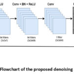Figure 1: Flowchart of the proposed denoising approach. Click here to view Figure

A concise explanation of the proposed method is illustrated in the steps below:

The step-by-step approach covers the major strategies of deep learning framework for denoising CT images, enabling the achievement of high-quality results while maintaining moderate computational intensity.³⁰Top of Form

Input: Noisy CT images.

Output: Denoised CT images.

Step 1: Dataset Preparation

Collect Dataset

The model takes a noisy image as input from a dataset, for example, the ELCAP Lung CT image Dataset. These images are often low-dose CT images (LDCT) that have been affected by Gaussian noise or other types of noise.

Preprocess Data

Standardize pixel intensities to make them manageable and easier to work with them. For example, scaling by dividing pixel values by 255 and multiplying by 2 results in a range of [-1, 1]). Resize all images to uniform dimensions, preferable sizes such as (256 x 256) or 512 x 512).

Data Augmentation

Apply basic data augmentation approaches, such as rotation, flipping and cropping, to expand the dataset and strengthen the model’s generalization.

Step 2: Build the DnCNN Model Network Architecture

DnCNN is a convolutional neural network that typically comprises the following components:

Input Layer: Initially, the input consists of noisy images.

Hidden Layers: The hidden layers comprise convolutional layers, such as-

Conv1 + ReLU : The first convolutional layer (3x3xnumber of channels) with (Rectified Linear Unit) ReLU is used for effective feature extraction by adding 64 kernels to each dimension. Here, the gray-scale images, the channel number is 1, and for color images, it is 3(RGB).

Conv2+BN+ReLU : From the second layer to the last layer, there is a combination of convolutional layers, typically around 17 layers in the DnCNN architecture, along with batch normalization (BN), and ReLU activation function. Each layer adds 64 filters to the dimensions 3x3x64. Batch normalization is applied between the convolutional and ReLU activation functions. Normalization is a preprocessing step of feature extraction, where pixel intensity values are scaled to a range of zero to one. Batch normalization helps to stabilize learning. The ReLU activation is used to provide nonlinearity into the neural network allowing it to analyze the input and help the network to learn complex structures in the data. Therefore, through hierarchical feature extraction and convolutional with ReLU, the CNN can successively separate noisy observation from the signal at various levels of its hidden layers.

 Step 3: Residual learning process

DnCNN effectively utilizes a residual learning approach, where the network automatically learns residuals i.e., the difference between the noisy image and the clean image. Each convolutional block includes a shortcut connection that adds the output of the convolutional layer to the original input CT image.

Step 4: Final Convolutional Layer

A Single convolutional layer (3x3x64) is used to reconstruct the denoised image.

Step 5: Final Output Layer:

The final denoised CT image is produced by subtracting the identified noise from the noisy input image. Consequently, the denoised image preserves crucial details while minimizing unwanted distortions. The DnCNN framework allows the network to capture noise patterns while preserving the clean CT image primarily unchanged.

Step 6: MSE Loss function:

Mean Squared Error (MSE) loss is used to minimize the disparity between the noisy and ground-truth images. It plays a key role in ensuring quality during the training process by providing a measure of how well the model performs in making its predictions.

MSE is evaluated by averaging the squared discrepancies among the pixel values of the noisy image and the clean image, defined as:

Where:

a_i​ denotes the pixel values of the noisy image,  is the pixel values of the clean image and N represents the total number pixels in the image.

For a grayscale image with dimensions M x N , the total number of pixels is expressed as:

N = M x N

Where M represents the number of rows i.e height of the image.

Where N represents the number of columns i.e width of the image.

For a color image with three channels (RGB), the total number of pixel values is expressed in MSE as:

M x N x C

Where C represents the number of channels (3 for RGB images and 1 for grayscale images).

The evaluation of images with more pixels exhibit lower Mean Squared Error (MSE) because error measurements are averaged across additional pixel values. Smaller images attenuate each pixel-wise error, resulting in a higher MSE value. The processing of images through resolution adjustments impacts MSE evaluation because downsampling tends to accumulate noise, while upsampling spreads it throughout the image. Therefore, the consistency of MSE comparison requires image samples with identical resolution.

Various optimization algorithms can be employed to optimize the model parameters and minimize the MSE loss. This enables the model to learn and improve overall imaging quality while suppressing noise.

Step 7: Stochastic Gradient Descent optimizer: Select an optimizer, such as the stochastic gradient descent, with an optimal learning rate, for example, a learning rate of 10^-4. Fine-tuning the model with appropriate SGD parameters can help it adapt to various CT image noise patterns, which may lead to better denoising performance.

SGD parameters include:

Learning Rate : Determines the size of weight updates. Common values are typically around 0.01 or 0.001.

Momentum: Helps to stabilize weight updates by incorporating a fraction of the previous update. A standard value of 0.9 is often used.

Weight Decay: Acts as a regularization technique to reduce the risk of overfitting. Typical

values range from 1e^-4 to 1e^-5.

Nesterov Acceleration: Enabling this option applies Nesterov Accelerated Gradient (NAG), which can enhance convergence rates during training. The convergence rate indicates how quickly an optimization algorithm determines the optimal solution, impacting training speed and model performance.

In practice, the DnCNN architecture consists of a deep convolutional network with batch-normalization, ReLU activations, and a number of convolutional layers in the form of residual learning. This structure enables the model to predict and estimate noise from various input images for denoising. By performing this process, noise is separated from the image, and important image features and structures are retained, which are beneficial to image denoising, making the DnCNN to deliver superior performance.

Results 

The Diagnostic evaluation was conducted on noisy grayscale CT images with 512 x 512-pixel dimensions. The test images for the CT scan test were acquired from a ELCAP  Lung CT image database to test the effectiveness of the proposed denoising method.³¹ The original CT images were required to assess the efficiency of the denoising algorithm. The reference clean CT image dataset is depicted in Figure 2, and Figure 3 shows the noisy CT-scan images are often degraded by gaussian noise at variance of σ =10. The deterioration in image quality is noticeable with the naked eye, in contrast to the clean CT image, even without the aid of image processing. The experimental outcomes of the proposed method’s quantitative analysis, in the context of PSNR, at σ=5,10,15,20 as depicted in Figures 4 to 7. Figure 8 shows the denoised CT images of the corresponding noisy CT1 image from Figure 3, with results are obtained from different denoising methods.

Quantitative analysis metrics

To evaluate the qualitative results obtained by the proposed methodology, the following methods like PSNR, SNR, SSIM and ED to measure the quality of denoised images.^32,33

PSNR is mainly used in evaluating the quality of recovered images with reference to the clean images. PSNR quantifies the relationship among the maximum signal strength provided and the power of the distorted image, that is the difference between the original image and the filtered-image. For the input CT image X_c and the denoised CT image Y_c.

PSNR is expressed as:

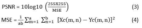
Where:

MSE depicts the mean squared error amongst the clean image and denoised image.

X_c (m, n) denotes the pixel value of the clean image at location (m, n).

Y_c (m, n) denotes the pixel value of the filtered image at location (m, n).

a x b illustrates the pixel dimensions of clean and a denoised image.

Signal-to-Noise ratio(SNR)

It is used to assess and determine the signal’s strength of interest with regard to the noise or disturbance occur in images. It is expressed in terms of decibels and is mainly used to measure the image quality.

P_signal is power of the signal, which represents the meaningful information, that is the desired information in the image.

P_noise stands for Power of noise interference which is typically random and unwanted signal that interferes with the quality of the signal.

Structural-Similarity-Index-Measure (SSIM)

It is a metric serves as a measure to evaluate the similarity among two images. It is primarily relying on 3 factors: contrast, luminance, and structural features, and the SSIM values vary between -1 and 1, where 1 specifies the exact similarity and -1 denotes variation between two images.

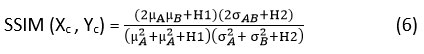
X_c denotes the clean image.

Y_c denotes the denoised image.

are described as the local means, ,  as standard deviations, and  is covariance of the clean image and denoised image X_c and Y_c Here, H1= , H2= are constants which are added to stabilize division by zero, where D represents the difference in pixel intensities values between  -1 and 1. Here, s1= 0.01 & s2 = 0.03.

Entropy difference (ED) 

It is the amount of randomness exist in an image in order to analyze the texture of the existed source images. Shannon entropy is calculated between clean (X_c ) and denoised image (Y_c) The difference in their respective mean values is represented as ED.

ED is defined as:

Where:

SE depicts the Shannon Entropy.

Shannon Entropy is calculated as:

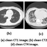Figure 2: Clean CT images; (a) clean CT1 image; (b) clean CT2 image; (c) clean CT3 image; (d) clean CT4 image.     Click here to view Figure

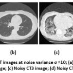Figure 3: Gaussian noisy CT images at noise variance σ =10; (a) Noisy CT1 image; (b) Noisy CT2 image; (c) Noisy CT3 image; (d) Noisy CT4 image. Click here to view Figure

The quantitative analysis confirms the efficacy of the proposed algorithm through comparisons with namely PSNR, SNR, SSIM and ED, as depicted in Tables 1 to 4 and Figures 4 to 7. These experimental outcomes suggest that the proposed method offers better overall performance than standard denoising methods. 

Table 1: PSNR values of the proposed approach with other compared methods.

Noise Variance ( σ )	5	10	15	20	5	10	15	20
Source CT Image	512 x 512				512 x 512
Total variation filter25	28.39	27.46	26.33	22.89	27.36	25.21	23.86	20.03
BM3D filter26	27.26	24.26	23.27	22.05	26.87	25.09	21.86	19.36
Guided filter27	26.95	25.88	25.65	24.46	27.75	26.13	23.34	22.58
Bilateral filter28	25.76	24.45	23.56	22.89	30.79	24.17	19.85	18.12
Anisotropic diffusion filter29	25.84	24.56	21.45	20.96	26.67	23.94	20.84	17.76
Proposed method	35.66	30.28	27.21	25.49	31.12	26.41	24.05	22.84

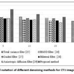Figure 4: Graphical notation of different denoising methods for CT1 image in terms of PSNR. Click here to view Figure

Table 2: SNR values of the proposed approach with other compared methods.

Noise Variance	5	10	15	20	5	10	15	20
Source CT Image	512 x 512				512 x 512
Total variation filter25	25.56	24.17	23.67	21.34	25.05	22.17	18.67	14.34
BM3D filter26	22.45	20.05	17.25	16.28	23.42	21.45	18.24	14.25
Guided filter27	22.15	22.08	21.83	21.07	21.98	19.23	15.85	13.68
Bilateral filter28	20.96	18.87	17.86	16.79	24.17	21.35	18.94	12.36
Anisotropic diffusion filter29	21.66	18.68	17.87	16.45	20.91	18.17	15.07	11.99
Proposed method	30.16	26.86	23.77	21.84	25.41	22.64	19.74	14.32

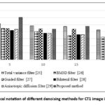Figure 5: Graphical notation of different denoising methods for CT1 image in terms of SNR. Click here to view Figure

Table 3: SSIM values of the proposed approach with other compared methods.

Noise Variance ( σ )	5	10	15	20	5	10	15	20
Source CT Image	512 x 512				512 x 512
Total variation filter25	0.8292	0.7174	0.6893	0.5678	0.8913	0.8655	0.8482	0.8538
BM3D filter26	0.7645	0.5753	0.5318	0.5065	0.9001	0.8753	0.7921	0.7645
Guided filter27	0.7045	0.6618	0.6068	0.5532	0.8976	0.8628	0.8456	0.8381
Bilateral filter28	0.8175	0.7688	0.7744	0.7496	0.8285	0.7688	0.7744	0.7496
Anisotropic diffusion filter29	0.8839	0.7866	0.5644	0.4587	0.8739	0.8366	0.8544	0.8387
Proposed method	0.9054	0.7932	0.7750	0.7416	0.9054	0.8932	0.87775	0.8616

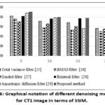Figure 6: Graphical notation of different denoising methods for CT1 image in terms of SSIM. Click here to view Figure

Table 4: ED values of the proposed approach with other compared methods.

Noise Variance ( σ )	5	10	15	20	5	10	15	20
Source CT Image	512 x 512				512 x 512
Total variation filter25	0.3675	0.4715	0.5466	0.6233	0.4685	0.5465	0.6166	0.7124
BM3D filter26	0.4944	0.7415	0.7532	0.8433	0.4944	0.6315	0.6532	0.7721
Guided filter27	0.4045	0.6677	0.7896	0.8256	0.4842	0.5966	0.6835	0.7676
Bilateral filter28	0.4469	0.6789	0.5433	0.6458	0.4469	0.6789	0.5433	0.6458
Anisotropic diffusion filter29	0.6978	0.7684	0.6523	0.7834	0.6978	0.7684	0.6523	0.7834
Proposed method	0.3555	0.4145	0.5587	0.6411	0.4321	0.5442	0.6023	0.6432

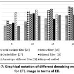Figure 7: Graphical notation of different denoising methods for CT1 image in terms of ED.Click here to view Figure

The proposed method yields significantly higher PSNR values at varying noise intensities (σ = 5,10,15,20) and shows better overall noise handling and image quality preservation abilities of CT1 image, as shown in Table 1. The proposed approach yields the higher PSNR values throughout the experiment, which is 35.66 dB for σ = 5 and 25.49 dB for σ = 20. On the other hand, the Total Variation and BM3D filters are effective at lower levels of noise as seen in the PSNR values of Total Variation 28.39 dB at σ = 5 and BM3D filter = 27.26 dB at σ = 5 respectively, but notable decline when it increases to σ = 20, with PSNR = 22.89 dB for Total Variation and PSNR = 22.05 dB perform less effectively as the noise intensity levels grow. The performance of the Total Variation filter can be improved at higher noise intensities by adapting regularization parameter based on the noise levels, which could enhance its denoising performance at higher noise levels. Compared to the other filters, Guided filter, Bilateral filter and Anisotropic Diffusion filter degrade CT1 image quality as noise level increase. Anisotropic Diffusion is the least effective, with performance dropping from 25.84 dB at σ = 5 to 20.96 dB at σ = 20.

 In the case of SNR values in Table 2, it is noted that Total Variation²⁵ has a slightly lower SNR value of 21.34 dB at a noise variance 20 compared to the proposed approach. The Total Variation method achieves enhanced Signal-to-Noise Ratio (SNR) measurements at a noise intensity of σ=20 by effectively smoothing homogeneous areas. However, it blurs both edges and detailed information, which results in a reduced Structural Similarity Index (SSIM). While it is effective for noise suppression, it compromises structural preservation properties better than the proposed method. However, classical techniques such as the bilateral filter, BM3D, and other filters experience limitations in both preserving fine details and managing severe noise levels, which can result in over smoothing. These filters are commonly used to evaluate the effectiveness of denoising tasks and also serve as a benchmark to assess the denoising performance of the proposed method. Overall, the proposed method achieves optimal efficiency under low noise levels and remains effective as the noise increases. Performance decreases gradually after noise levels σ = 25 or 30 but shows superior results when compared to conventional filter methods.

In the proposed method, SSIM values remain consistently high even as noise intensity levels increase, indicating that it effectively preserves structural details to improve image quality. It is noticed that the proposed approach gives the highest SSIM values throughout a wide range of noise variances with a minimum of 0.74. The experimental data depicts that both the total variation filter and BM3D filter have relatively lower precision compared to other filters and the precision decreases as the noise level increases. Here, the proposed method is superior to the other filters in terms of image quality preservation. Overall, the method shows higher SSIM values for CT1 image, indicating better structural preservation, as depicted in Table 3. By evaluating the results for various noise intensity levels, the proposed method yields the lowest ED values, indicating its effectiveness in preserving edge details of the image, as shown in Table 4. On the other hand, the proposed method shows lower ED values compared to BM3D and the Anisotropic Diffusion filter because it effectively minimizes noise while preserving edges and textures. Unlike BM3D, which introduces artifacts and anisotropic diffusion, which causes excessive smoothing that affect edges, these methods show higher ED values, indicating that they retain fewer edge details as the noise variance increases. The proposed method leverages a deep learning framework to extract complex noise patterns, preserving high image quality without manual parameter tuning. The proposed method, leveraging DnCNN outperforms conventional filters like BM3D and Anisotropic diffusion. Overall, from Tables 1 to 4, it is clear that the proposed method yields better denoising quality-based outcomes.

Qualitative analysis

Qualitative analysis of the experimental outcomes contaminated with Additive White Gaussian noise.

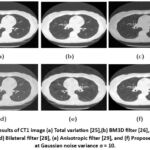Figure 8: Results of CT1 image (a) Total variation [25],(b) BM3D filter [26], (c) Guided filter [27], (d) Bilateral filter [28], (e) Anisotropic filter [29], and (f) Proposed approach at Gaussian noise variance σ = 10.Click here to view Figure

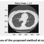Figure 9: PSNR values of the proposed method at noise variance σ = 5.Click here to view Figure

Figure 10: PSNR values of the proposed method at noise variance σ = 10.Click here to view Figure

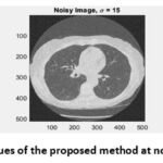Figure 11: PSNR values of the proposed method at noise variance σ = 15.Click here to view Figure

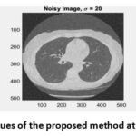Figure 12: PSNR values of the proposed method at noise variance σ = 20.Click here to view Figure

The region of 45 × 45 pixels in the upper right quadrant of the CT images was selected for a zooming analysis of the details such as edges, contrast and different shades of grayscale images, as shown in Figures 13 and 14. The specified region was identified and outlined in all the noisy and denoised CT scan images using MATLAB2022b. As in Figure 15, the zoomed-in analysis of the marked regions highlights the remarkably high edge reconstruction and contrast recovery in the white detail areas of the denoised CT images.

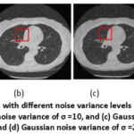Figure 13: Noisy CT images with different noise variance levels (a) Gaussian noise variance of σ =5 , and (b) Gaussian noise variance of σ =10, and (c) Gaussian noise variance of σ =15, and (d) Gaussian noise variance of σ =20.Click here to view Figure

Figure 14: Denoised CT images of Proposed technique and marked region is used for zooming analysis of the marked-region;(a) Gaussian noise variance level σ =5, and (b) Gaussian noise variance level σ =10, and (c) Gaussian noise variance level σ =15, and (d) Gaussian noise variance level σ =20.Click here to view Figure

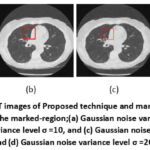Figure 15: Comparison of zooming analysis of the marked region of noisy and proposed denoised CT1 image;(a) Gaussian noise variance level σ =5, and (b) Gaussian noise variance level σ =10, and (c) Gaussian noise variance level σ =15, and (d) Gaussian noise variance level σ =20.Click here to view Figure

The intensity profile in CT images depicts how pixel intensities change along a specific path, helping to assess contrast, consistency, and noise intensity levels in the image. It helps to determine image quality, identify structural edges, and analyze noise in CT images. The intensity profile is employed to evaluate the CT image quality by noting the pixel density corresponding to the grayscale images. The similarity among two CT images can be identified by comparing their intensity profile plots. In this case, the method is used to assess how closely the denoised image resembles the clean image by comparing the pixel values of different locations. Figure 17 shows the intensity profile of the CT1 image at varying noise levels (σ = 5,10,15,20) respectively. The results indicate that the denoised and original CT images share significant similarities, proving the efficiency of the adopted denoising method in maintaining image quality. Other experiments conducted at different noise levels, as presented in this paper, further confirm the reliability of the proposed system.

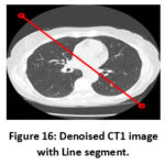Figure 16: Denoised CT1 image with Line segment.Click here to view Figure

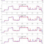Figure 17:Intensity profile of a line on clean image and denoised CT1 image of various denoising methods from [25-29].Click here to view Figure

The intensity profile of²⁵ deviates more at the edges and sharp transitions compared to the proposed approach, due to the staircase effect and²⁶ efficiently reduces noise but compromises edges and fine structures slightly, resulting in mild blurring. The intensity profile of²⁷ preserves smooth surfaces but slightly reduces texture changes, leading to compression of fine details. The intensity profile of²⁸ is effective in removing noise, but it has the disadvantage of blurring, particularly around edges, which distorts the fine details and²⁹ is also very similar to the one as shown in²⁸, as it also sacrifices fine detail while attempting to eliminate noise. Conversely, the proposed approach maintains the intensity profile of the clean image thereby providing better noise mitigation and superior retention of edges and fine details as compared with conventional techniques.

Discussion

The efficiency of the proposed ensemble method was assessed using PSNR, SNR, SSIM and ED metrics. The performance assessment of the DnCNN model for denoising CT images is demonstrated the efficiency and the importance of noise removal to enhance imaging quality. The proposed ensemble approach is compared with different benchmarks like PSNR, SNR and SSIM and ED. The proposed ensemble method, effectively utilizing DnCNN framework, achieved outstanding results in denoising CT images compared to conventional denoising techniques. It obtained higher PSNR and SNR values, indicating effective noise suppression while preserving fine image details. The SSIM results depict enhanced structural retention, while lower ED values indicate improved edge preservation. Compared to conventional denoising techniques, the DnCNN approach excels in both noise suppression and fine detail preservation. PSNR measures the denoised image quality in comparison with original noisy image. The higher PSNR represents the greater fidelity. It is measured in decibels (dB). The SNR examines the strength of preferred signal with the level of background noise. The range of SSIM values in between 0 and 1 i.e., 1 depicts the complete resemblance to the original image and denoised image. Whereas 0 depicts there is no structural similarity between denoised image and clean image.

The quantitative assessment values of the CT1 image at different noise intensities show that the proposed method achieves the highest PSNR value, indicating superior noise mitigation while preserving fine image details. At (σ=10), the proposed model achieves 30.28 dB, performs better than BM3D, which has a PSNR value of 24.26 dB, and Total Variation, which achieves 27.46 dB, achieving robustness in moderate noise levels. Total variation and Anisotropic diffusion depict lower PSNR values as noise increases, reducing denoising performance in LDCT images. Total Variation, Bilateral, and Guided filters result in excessive smoothing, degrading image quality at higher noise intensities compared to the proposed approach. This highlights the effectiveness of the proposed method in noise suppression and detail preservation.

For SNR, the proposed method shows strong signal retention even at higher noise levels. It outperforms BM3D and Total Variation at (σ = 10), achieving an SNR value of 26.86 dB, compared to their 20.05 dB and 24.17 dB results. The signal retention of the proposed method remains at 23.77 dB when (σ =15), while BM3D and Anisotropic Diffusion decrease to 17.25 dB and 17.87 dB, respectively. Traditional denoising methods such as Anisotropic Diffusion, Bilateral and BM3D shows abrupt SNR deterioration as noise increases, resulting in a severe drop in CT image quality. The proposed method achieves an SSIM value is of 0.7932 under a noise variance (σ = 10), whereas BM3D exhibits 0.5753 and Total Variation reaches 0.7174. The proposed method obtains an SSIM value of 0.7750 as σ approaches 15, remaining higher than BM3D, which has a value of 0.5318, indicating significant structural disruption to image quality. With a noise variance (σ = 15), the structural integrity preservation of Anisotropic Diffusion becomes difficult, as its SSIM value drops to 0.5644, highlighting its struggle to preserve vital anatomical features.

The proposed method achieves the lowest entropy difference (ED) values, indicating effective edge preservation. At a noise level of (σ = 10), it attains an ED value of 0.4145, outperforming BM3D’s 0.7415 and Anisotropic Diffusion’s 0.7684. Even at (σ = 15), it maintains an ED value of 0.5587, while BM3D rises to 0.7532, representing a greater loss of edge details. In contrast, traditional filters such as Total Variation, Anisotropic Diffusion, and Bilateral filters exhibit higher ED values, indicating their tendency to obscure fine details. Overall, the experimental results confirm that the proposed DnCNN-based model outperforms other denoising techniques in higher noise environments such as low dose CT imaging, where both noise suppression and fine detail preservation are essential to improve image quality. The proposed method can be adapted to different domain specific datasets such as diverse medical image datasets, to extract specific features like organ structures, lesions, and tissues through fine-tuning the DnCNN model. It can also be adjusted to varying noise levels using custom-loss functions and data augmentation.

An intensity profile represents the distribution of pixel values in an image, emphasizing changes in contrast and fine detail. The intensity profiles of the clean image with various standard denoising methods and clean image with proposed method illustrate superior noise suppression while effectively maintaining intricate details, leading to more precise edges and clearer transitions, as shown in Fig. 17. Overall, proposed approach shows high accuracy and computational efficiency, compared to the other standard denoising methods.

Future research Work

In future work, the proposed DnCNN can incorporate domain-specific priors to preserve diagnostic features more effectively. Future research work may extend the proposed hybrid models with attention blocks to achieve better results for more complex noise patterns. Generalizing the model for Poisson or mixed noise will enhance its versatility for low-dose CT imaging in practice. Real-time optimizations and validations on multiple clinical databases are essential for accurate medical diagnosis of various diseases.

Conclusions

This research proves that the proposed approach based on DnCNN yields better results for Gaussian noise reduction in CT images than traditional filters. The outcomes of the proposed deep learning-based method were compared with PSNR, SNR, SSIM and ED metrics, and the results showed higher efficiency against other techniques such as Total Variation filter,²⁵ BM3D filter,²⁶ Guided filter,²⁷ Bilateral filter,²⁸ and Anisotropic Diffusion filter.²⁹ Unlike conventional methods, which rely on prior knowledge in terms of models or assumptions about the type of noise distribution, the DnCNN learns from the data and can effectively handle a variety of noise levels. The deep convolutional network is successfully utilized to learn and selectively remove noise while reconstructing the fine structures of the given CT image without over-smoothing it. By utilizing deep convolutional layers, the model is trained to concentrate on residual noise instead of directly denoising the whole image. The proposed method outperforms traditional denoising filters by achieving higher PSNR and SNR values, ensuring effective noise mitigation while preserving fine image details. The method maintains better structural preservation (SSIM) compared to Total Variation, BM3D, Guided filter, and Anisotropic diffusion, which degrade at higher noise intensities. The proposed method also shows lower ED values, resulting superior edge retention and prevention of over-smoothing. Overall, the proposed method provides an optimal balance of noise suppression, edge and structure preservation, resulting in enhanced CT image quality.

The proposed method is adaptable to various medical imaging modalities, including CT, X-ray, MRI, and ultrasound. Through customization of the model with specific datasets, it can adapt to distinct noise patterns, effectively mitigating noise while preserving fine image details. This leads to enhanced diagnostic accuracy by increasing the perceptibility of critical image features, ultimately increasing reliability in medical diagnosis. Therefore, the proposed method provides a benchmark for denoising of CT images in medical diagnosis, aiming to enhance reliability and accuracy. 

Acknowledgement

I express my heartfelt gratefulness to Prof. Deepak Garg, SR University, Telangana and Dr. Prabhishek Singh, Bennett University, Noida, for their significant insight, support and assistance during this study. I also express my gratitude to Prof. Manoj Diwakar from Graphic Era University, Dehradun, for his significant support and informative feedback, which profoundly elevated the quality of this reach work.

Funding Source

The author(s) received no specific funding for this research work.

Conflicts of Interest

The author(s) state no conflicts of interest. 

Data Availability Statement

This statement does not apply to this article.
Ethics Statement

This research did not involve human participants, animal subjects, or any material that requires ethical approval.
Informed Consent Statement

This study did not involve human participants, and therefore, informed consent was not required.
Clinical Trial Registration

This research does not involve any clinical trials

Author Contributions

Swapna Katta: Conceptualization, Data Collection, Methodology, Writing the draft, software, coding, Validation.

Prabhishek Singh: Analysis, Visualization, Writing review and Editing.

Deepak Garg: Investigation, Supervision, Visualization.

Manoj Diwakar: Validation and Visualization.

References

1. Ziyad SR, Radha V, Vaiyapuri T. Noise removal in lung LDCT images by novel discrete wavelet-based denoising with adaptive thresholding technique. Int J E-Health Med Commun (IJEHMC). 2021;12(5):1-15.
   CrossRef
2. Zubair M, Rais HM, Alazemi T. A novel attention-guided enhanced U-Net with hybrid edge-preserving structural loss for low-dose CT image denoising. IEEE Access.
   CrossRef
   
3. Oh J, Wu D, Hong B, Lee D, Kang M, Li Q, Kim K. Texture-preserving low-dose CT image denoising using Pearson divergence. Phys Med Biol. 2024;69(11):115021.
   CrossRef
4. Zhang J, Gong W, Ye L, Wang F, Shangguan Z, Cheng Y. A review of deep learning methods for denoising of medical low-dose CT images. Comput Biol Med. 2024;108112.
   CrossRef
5. Zubair M, Rais HM, Al-Tashi Q, Ullah F, Faheeem M, Khan AA. Enabling predication of the deep learning algorithms for low-dose CT scan image denoising models: A systematic literature review. IEEE Access. 2024.
   CrossRef
6. Nazir N, Sarwar A, Saini BS. Recent developments in denoising medical images using deep learning: an overview of models, techniques, and challenges. 2024;103615.
   CrossRef
7. Sadia RT, Chen J, Zhang J. CT image denoising methods for image quality improvement and radiation dose reduction. J Appl Clin Med Phys. 2024;25(2):e14270.
   CrossRef
8. Zhao H, Zhu Y, Yao Y. Low-dose CT image denoising based on residual attention mechanism. In: Proceedings of the Sixth International Conference on Information Science, Electrical, and Automation Engineering (ISEAE 2024). Vol 13275. SPIE; 2024:328-333.
   CrossRef
9. Ding S, Wang Q, Guo L, Zhang J, Ding L. A novel image denoising algorithm combining attention mechanism and residual UNet network. Knowl Inf Syst. 2024;66(1):581-611.
   CrossRef
10. Wang Y, Yang N, Li J. GAN-based architecture for low-dose computed tomography imaging denoising. arXiv preprint arXiv:2411.09512.
    
11. Li Q, Li R, Li S, Wang T, Cheng Y, Zhang S. Unpaired low-dose computed tomography image denoising using a progressive cyclical convolutional neural network. Med Phys. 2024;51(2):1289-1312.
    CrossRef
12. Li H, Yang X, Yang S, Wang D, Jeon G. Transformer with double enhancement for low-dose CT denoising. IEEE J Biomed Health Inform. 2022;27(10):4660-4671.
    CrossRef
13. Mahmoodian N, Rezapourian M, Inamdar AA, Kumar K, Fachet M, Hoeschen C. Enabling low-dose in vivo benchtop X-ray fluorescence computed tomography through deep-learning-based denoising. J Imaging. 2024;10(6):127.
    CrossRef
14. Diwakar M, Kumar M. A review on CT image noise and its denoising. Biomed Signal Process Control. 2018;42:73-88.
    CrossRef
15. Annavarapu A, Borra S. An adaptive watershed segmentation based medical image denoising using deep convolutional neural networks. Biomed Signal Process Control. 2024;93:106119.
    CrossRef
16. Oh J, Wu D, Hong B, Lee D, Kang M, Li Q, Kim K. Texture-preserving low dose CT image denoising using Pearson divergence. Phys Med Biol. 2024;69(11):115021.
    CrossRef
17. Saidulu N, Muduli PR, Dasgupta A. RHLNet: Robust hybrid loss-based network for low-dose CT image denoising. IEEE Trans Instrum Meas.
    CrossRef
    
18. Huang J, Chen K, Ren Y, Sun J, Pu X, Zhu C. Cross-domain low-dose CT image denoising with semantic preservation and noise alignment. IEEE Trans Multimedia.
    CrossRef
    
19. Niknejad Mazandarani F, Babyn P, Alirezaie J. Low-dose CT image denoising with a residual multi-scale feature fusion convolutional neural network and enhanced perceptual loss. Circuits Syst Signal Process. 2024;43(4):2533-2559.
    CrossRef
20. Jin H, Tang Y, Liao F, Du Q, Wu Z, Li M, Zheng J. Adaptive noise-aware denoising network: Effective denoising for CT images with varying noise intensity. Biomed Signal Process Control. 2024;96:106548.
    CrossRef
21. Kumrular RK, Blumensath T. Unsupervised denoising in spectral CT: Multi-dimensional U-Net for energy channel regularisation. 2024;24(20):6654.
    CrossRef
22. Tiantian W, Hu Z, Guan Y. An efficient lightweight network for image denoising using progressive residual and convolutional attention feature fusion. Sci Rep. 2024;14(1):9554.
    CrossRef
23. Zhang K, Niu T, Xu L. DeCoGAN: MVCT image denoising via coupled generative adversarial network. Physics in Medicine & Biology. 2024;69(14):145007.
    CrossRef
24. Song Q, Li X, Zhang M, Zhang X, Thanh DN. APNet: Adaptive projection network for medical image denoising. J X-Ray Sci Technol. 2024;1-15.
    CrossRef
25. Bai T, Wang B, Nguyen D, Jiang S. Probabilistic self-learning framework for low-dose CT denoising. Med Phys. 2021;48(5):2258-2270.
    CrossRef
26. Diwakar M, Singh P, Swarup C, Bajal E, Jindal M, Ravi V. Noise suppression and edge preservation for low-dose COVID-19 CT images using NLM and method noise thresholding in shearlet domain. 2022;12(11):2766.
    CrossRef
27. Diwakar M, Singh P, Garg D. Edge-guided filtering-based CT image denoising using fractional order total variation. Biomed Signal Process Control. 2024;92:106072.
    CrossRef
28. Diwakar M, Kumar P. Wavelet packet-based CT image denoising using bilateral method and Bayes shrinkage rule. In: Singh A, Mohan A, Kumar N, eds. Handbook of Multimedia Information Security: Techniques and Applications. Springer; 2019:501-511.
    CrossRef
29. Chen Y, Dai X, Duan H, Gao L, Sun X, Nie S. A quality improvement method for lung LDCT images. J X-Ray Sci Technol. 2020;28:255-270.
    CrossRef
30. Singh P, Diwakar M, Gupta R, Kumar S, Chakraborty A, Bajal E. A method noise-based convolutional neural network technique for CT image denoising. 2022;11(21):3535.
    CrossRef
31. Sagheer SVM, George SN. A review on medical image denoising algorithms. Biomed Signal Process Control. 2020;61:102036.
    CrossRef
32. Li Z, Zhou S, Huang J, Yu L, Jin M. Investigation of low-dose CT image denoising using unpaired deep learning methods. IEEE Trans Radiat Plasma Med Sci. 2020;5(2):224-234.
    CrossRef
33. Charatpangoon P, Delannoy P, McDougall C, et al. Radiation dose reduction in computed tomography perfusion of acute ischemic stroke patients using a denoising autoencoder. In: 2024 IEEE International Symposium on Biomedical Imaging (ISBI); May 2024; IEEE; 2024:1-5.
    CrossRef