Karan Kumar¹, Isha Suwalka^2*, Harishchander Anandaram³ and Kapil Joshi⁴

¹Electronics and Communication Engineering Department, Maharishi Markandeshwar Engineering College, Maharishi Markandeshwar (Deemed to be University), Mullana, Ambala, India

²Department of Research and Publication, Indira IVF Hospital Limited, Udaipur, India

³Department of Artificial Intelligence, Amrita Vishwa Vidyapeetham, Coimbatore, Tamil Nadu, India.

⁴Department of Computer Science and Engineering, Uttaranchal Institute of Technology (UIT), Uttaranchal University, Dehradun, Uttarakhand, India.

Corresponding Author E-mail:suwalkaisha3@gmail.com

DOI : https://dx.doi.org/10.13005/bpj/3074

Abstract

Brain tumor detection from MRI images is crucial for early diagnosis and treatment. Various clustering algorithms, such as Fuzzy K-means (FKM), Fuzzy C-means (FCM), and Self-Organizing Maps (SOM), have been used for segmentation, but they face challenges like noise and varying image intensities. This study evaluates the performance of the Adaptive Moving Self-Organizing Map (AMSOM) for tumor segmentation in MRI images, comparing it to other clustering methods. We evaluated FCM, FKM, SOM-FKM, and AMSOM on a dataset of 12 MRI images. Performance was measured using Peak Signal-to-Noise Ratio (PSNR), accuracy, Mean Square Error (MSE), and similarity criteria. AMSOM outperformed other methods with an MSE of 0.01, PSNR of 68.16 dB, accuracy of 89.11%, and similarity criteria of 96.8%. In comparison, FCM showed an MSE of 2.880 and PSNR of 43.57 dB, while FKM had an MSE of 1.9 and PSNR of 45.17 dB. AMSOM provides superior segmentation accuracy and computational efficiency, making it a highly effective approach for detecting brain tumors in MRI images. Its robust performance highlights its potential for medical imaging applications. Future research could expand its use to include PET scans and 3D imaging, enabling broader applicability in advanced medical diagnostics and treatment planning.

Keywords

AMKFSOM; Brain Tumor; clustering; feature extraction; Magnetic Resonance Imaging

Download this article as: 

Copy the following to cite this article: Kumar K, Suwalka I, Anandaram H, Joshi K. An Automatic Simulation of MRI using Adaptive Unsupervised Mapping. Biomed Pharmacol J 2025;18(March Spl Edition).

Copy the following to cite this URL: Kumar K, Suwalka I, Anandaram H, Joshi K. An Automatic Simulation of MRI using Adaptive Unsupervised Mapping. Biomed Pharmacol J 2025;18(March Spl Edition). Available from: https://bit.ly/41vpICA

Introduction

A tumor is an uncontrolled growth of cells in the brain, typically identified using various imaging techniques, among which MRI is the most common. MRI provides a complete image of the brain but faces several challenges, such as manual reorientations, visual evaluations, and other time-consuming errors. Statistical data from developed countries tells that people often die due to inaccurate and late-stage predictions of tumors.¹

Brain tumors can be benign and malignant. Benign tumors are non-cancerous, grow at a controlled rate, and do not affect surrounding cells. These tumors are usually easy to identify, remove, and rarely grow back. On the other hand, malignant tumors grow rapidly, contain cancerous cells, and require early diagnosis to improve survival chances. Tumor segmentation involves partitioning the surrounding healthy brain tissue. However, imaging techniques often struggle to accurately identify tumor locations and boundaries, leading to misidentification and misinterpretation. MRI images, which provide visual representations of the brain’s interior, often suffer from issues such as noise, low contrast, and poor homogeneity. These problems can be critical when performing clinical analysis and making medical decisions. Therefore, there is a need for efficient algorithms that act as fully automated systems for analyzing MRI images for diagnostic purposes.²

The author Somasundaram applied an algorithm for axial T2-weighted images. Another author used SVM classifier for tumor detection, while many researchers have utilized optimization techniques for feature reduction.

In this research, we employ a method that is more effective than the usual techniques, combined with FKM and Gray-Level Co-occurrence Matrix (GLCM). We compare the proposed method with FCM, FKM, and SOM based on several evaluation metrics, including accuracy, MSE, PSNR, Tanimoto index, and Dice coefficient, which are defined in later sections. The comparison of various mapping methods and their parameters is emphasized. The calculations were done on MATLAB. The following sections explain the concepts and processing steps involved.

Literature Review

In recent years, significant progress has been made in brain tumor segmentation and detection from MRI data. Many techniques have been developed to enhance the efficiency and accuracy of tumor detection, which plays a crucial role in disease diagnosis and treatment planning. Several studies have explored the effectiveness of these methods in both unsupervised and supervised learning contexts.

The Dasgupta et al² provided a comprehensive summary of the data on central nervous tumors in India, detailing various methods used for the identification and diagnosis of these tumors using imaging techniques. Their work highlights the regional challenges and the increasing reliance on MRI for accurate brain tumor detection, noting that the development of more sophisticated computational techniques is vital for early and accurate diagnosis in Indian clinical settings.

The Govindaraj et al³ emphasized the application of unsupervised learning techniques, such as clustering, in tumor identification and tissue segmentation. Their study showed the promising role of clustering methods like FCM and SOM in MRI brain image analysis. These techniques help in distinguishing abnormal brain tissue, which is crucial for accurate diagnosis and treatment. In a similar vein, the Nandhagopal and Ganesh⁴ explored automatic brain tumor detection through MRI using unsupervised learning, focusing on overcoming the challenges posed by noise and variability in the images.

Markov Random Fields (MRF) have been successfully applied in medical image segmentation. The Guerrout et al⁵ employed MRF for segmentation in a cluster of PCs, demonstrating that MRF could significantly improve the quality of segmentation by modelling the spatial dependencies between neighboring pixels. This method was particularly beneficial in medical imaging, where the precise delineation of tumor boundaries is essential for accurate diagnosis and treatment planning.

The Ortiz et al⁶ proposed unsupervised methods for segmenting the MRI brain image. Their methods demonstrated effectiveness in brain tumor segmentation by adapting the SOM framework to handle varying intensities in MRI images. The integration of SOM-based strategies helped in reducing the complexity of segmentation tasks without requiring labelled data, thus making it applicable for large-scale clinical applications.

Fuzzy clustering methods have become increasingly popular for medical image segmentation due to their ability to handle uncertainty and noise in imaging data. Aljahdali and Zanaty⁷ explored the use of fuzzy clustering algorithms for automatic image segmentation. They noted that fuzzy methods are particularly useful in medical imaging, where pixel intensities can overlap between healthy and abnormal tissues, thus improving tumor segmentation accuracy. Furthermore, the Vasuda and Satheesh⁸ proposed an updated version of FCM for MR brain image segmentation, which sought to overcome the limitations of traditional FCM, especially in noisy images.

Support Vector Machines (SVM) have also been widely applied for tumor classification. The Abdi et al⁹ introduced a novel weighted SVM method for gene selection and tumor classification, showing its potential for effective tumor detection and classification in medical imaging. By optimizing feature selection, SVM can improve the classification accuracy in high-dimensional data, making it an important tool for brain tumor detection.

The Abdel-Maksoud et al¹⁰ developed a technique for brain tumor segmentation, which combined multiple clustering approaches to improve segmentation accuracy. Their hybrid method showed that combining different clustering algorithms could effectively handle varying image characteristics, leading to more accurate tumor detection and segmentation. This approach complements the advances made by other hybrid techniques such as AMSOM, proposed by the Spanakis and Weiss¹¹. AMSOM enhances traditional SOM by incorporating adaptive learning strategies, improving clustering and visualization, and thus providing better segmentation for medical images. K-means clustering is another popular algorithm for image segmentation. The Dhanachandra et al¹² compared K-means with subtractive clustering algorithms for MRI image segmentation, noting that subtractive clustering provided superior performance in handling complex images with varying intensities. This study demonstrated that by selecting the appropriate clustering algorithm, the quality of segmentation can be significantly improved, aiding in more accurate tumor detection. Finally, the Roy et al¹³ proposed an iterative level set approach for abnormality detection and precise segmentation of brain tissues from MRI images. This technique proved effective in accurately delineating brain tumors from surrounding tissues, thus enabling better detection of abnormalities and enhancing the clinical utility of MR images.

Materials and Methods

Self Organizing Map (SOM)

SOM are a widely used technique in unsupervised learning, known for their efficiency in organizing high-dimensional data. SOM organizes similar feature vectors into a two-dimensional (or higher-dimensional) lattice, which is mapped onto an output space. The structure of SOM is defined by a set of neurons and a distance vector that influences the arrangement and weight factors within the map. During the training, the input data is used to calculate the distance between each input and the corresponding weight factors, and the neurons are mapped from a high input space to a lower plane. An important parameter is the Best Matching Unit (BMU), which is updated during training to improve the map’s accuracy.^14,15

The primary objective of SOM is to organize high-dimensional data into a lower-dimensional, typically two-dimensional, grid. This is done by mapping similar input data points together, creating a map where each neuron in the grid represents a specific pattern or feature of the input data. Each input vector 𝑥(𝑡)=[𝑥₁, 𝑥₂,…,𝑥_𝑀], where 𝑡=1,2,…,𝐿, represents a set of 𝑀 features. These features are connected to all neurons in the network through their respective weight vectors 𝑤_𝑗=[𝑤₁,𝑤₂,…,𝑤_𝑁]. Here, 𝑖=1 to 𝐿 denotes the input instances, and 𝑗=1,2,…,𝑀 corresponds to the number of neurons. Each feature in the input vector is processed by the neurons through these weights, enabling the model to learn relationships and patterns. The neuron closest to the input vector is identified as the BMU, which is calculated by determining the neuron that minimizes the Euclidean distance of all the neurons. This is given by:

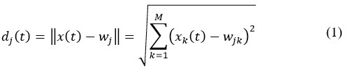
where   represents the Euclidean distance between the input vector 𝑥(𝑡) and the weight vector 𝑤𝑗 associated with neuron 𝑗 at a specific time step 𝑡. This distance is a measure of how similar or different the input vector is from the neuron’s weight vector. The neuron with the smallest distance, , is chosen as the BMU:

Adaptive Moving Fuzzy K-means Self Organizing Map (AMFKSOM)

The algorithm includes integration of two algorithm AMSOM and FKM. The proposed method follows following steps^16,17:

Set up a rectangular grid to represent the network, where each point on the grid corresponds to a neuron. The number of neurons, 𝑁, defines the grid’s dimensions and structure.

Initialize weight vectors (wp) randomly: Assign random initial values to the weight vectors 𝑤_𝑝 based on the number of features in the data, following a similar process as the SOM batch algorithm. At each epoch 𝑠, the weight vector 𝑤_𝑣(𝑠+1) is updated for the next epoch. The number of input patterns assigned to neuron 𝑢 is represented by 𝑛𝑢(𝑠), while the neighborhood function 𝜃(𝑢,𝑣,𝑠) measures the proximity between neuron 𝑢 and its neighboring neuron 𝑣. The feature vector 𝑥_𝑢(𝑠) is the mean of all input patterns assigned to neuron 𝑢. The adaptation factor 𝜎(𝑡) decreases during training, controlling the degree of weight adjustments and ensuring that the network adapts gradually. So 

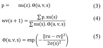
Lastly, the w_u are figured when the neuron weight vectors update is over.¹⁸

Initialize position vectors (remove_p1) acc. to (8 or 10) grid structure.

Initialize the edge connectivity matrix (Eg): Set the values based on the grid structure, defining the connectivity between neighboring neurons.

Initialize the edge age matrix (Ag): Set all values to zero, indicating that no connections have been established yet

Compute the moving threshold (MT) based on the dimensionality of the data derived from the GLCM and then compute spreading factor (SF). It is given by

Find the winner neuron (N): During the training phase, identify the neuron 𝑁 that best matches the input. Increment the winning neuron’s count by 1 to signify its selection as the winner.

Find the second-best matching neuron (Nb): Identify the neuron 𝑁_𝑏 that is the second-best match, excluding the winner neuron 𝑁.

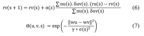
Age all edges between 𝑁 and its neighbors: Increment the age of all edges connected to the winner neuron 𝑁 and its neighboring neurons. The age of each edge increases by 1, reflecting the duration of the connection. If the age of an edge 𝐴(𝑖,𝑗) between neurons 𝑖 and 𝑗 exceeds a predefined maximum age threshold (𝑎𝑔𝑒𝑚𝑎𝑥), then the edge is removed from the network, indicating the disconnection of outdated or less relevant connections.

Establish a connection between neuron 𝑁 and its neighboring neuron 𝑁_𝑏.

Reset the edge weight between 𝑁 and 𝑁_𝑏 to zero to initiate the update process.

Update the neuron weights and positions based on the input feature vectors and competitive learning rules.

Recompute and adjust the position of each neuron to better represent the feature space.

Determine whether additional neurons need to be added or existing ones removed, and update the network structure accordingly to maintain optimal performance.

Check for convergence by monitoring the error change. If the error does not change significantly, proceed to end Step 7. Otherwise, continue the iterative process to refine the network.

Enter the smoothing phase, where the neuron weight vectors undergo fine-tuning to enhance precision. The final output is the optimized AMSOM neuron weight vectors, ensuring robust and accurate clustering of the input data.

Feed the centroid to compute clustering using K means using

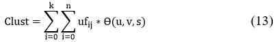
In our system, we leverage the benefits of two algorithms: one that accelerates the clustering of regions and another that efficiently classifies the data using mapping. As illustrated in Figure 1, the system consists of five stages: pre-processing, clustering, feature extraction, classification, and validation. The core idea behind this technique is to reduce the number of iterations and the dimensionality of the data,^19,20 which, in turn, reduces computational time and enhances efficiency. Feature extraction plays a critical role by identifying distinctive properties from the original dataset that generate unique patterns.

The feature vector for MRI images is calculated using both first-order and second-order features derived from the covariance matrix. Table 1 lists the specific features used.

Pre-processing steps are a critical part of preparing MRI images for analysis, as they ensure the input data is clean and standardized, thereby enhancing the accuracy and reliability of subsequent processing stages. For the proposed method, preprocessing includes two major steps: skull removal and denoising. Skull removal isolates the brain region from non-relevant structures, focusing the analysis solely on the area of interest. Denoising addresses various types of corrupted noise commonly present in MRI images, such as Gaussian and Poisson noise, which can distort the image quality and affect the accuracy of downstream processes.

Once preprocessing is complete, the clustering stage begins. The extracted feature vectors from the preprocessed images are input into a hybrid clustering framework that combines Fuzzy K-means (FKM) and Adaptive Self-Organizing Maps (AMSOM). AMSOM is initially employed for clustering and dimensionality reduction, effectively simplifying the high-dimensional data from MRI images while preserving critical information.

For this process, the real brain images, acquired from hospitals, are resized to a uniform 256×256 pixel format to ensure consistency across datasets. AMSOM then reduces the dimensionality of the resized images, preparing them for further clustering refinement by FKM. This combination of preprocessing and advanced clustering techniques ensures high segmentation accuracy, efficient computational performance, and robust handling of complex medical imaging datasets. In this process, random vectors are initially assigned as weight factors for the neurons. The neurons compete to identify a “winning neuron” for each input, which is determined based on these weights. The competition is guided by the calculation of the Euclidean distance between the input vector and the weight vectors of the neurons. The AMSOM algorithm then updates the weight function, which is subsequently passed to the FKM algorithm for further clustering refinement, ensuring enhanced accuracy and representation of the MRI data. The inclusion of AMSOM mitigates the limitations of FKM when handling large datasets, making the system more efficient and effective. Figure 1 illustrates the block diagram of the methodology employed in our proposed system.

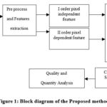Figure 1: Block diagram of the Proposed method     Click here to view Figure

During the validation phase, the segmented images are evaluated against the ground truth using the equations provided in the experimental results.

These values are dimensionless but can be expressed as percentages by multiplying them by 100.

Mean Square Error (MSE) is a quantitative measure used to assess the difference between the input image 𝑀(𝑖,𝑗) and the segmented image 𝑆(𝑖,𝑗).²¹ It is given by

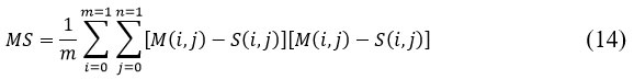
where ‘m’ & ‘n’ denotes the matrix size in an input image.

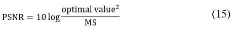
PSNR is defined as the logarithmic ratio between the maximum possible signal power and the power of the noise affecting the image. The PS values less sensitive to noise signals lies between 40 to 100 dB. PSNR is given by:

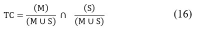
The Tanimoto Index (TC), also known as the Jaccard Index, is a similarity measure used to evaluate the accuracy of segmentation by comparing the input image (M) with the segmented output image (S).

The Dice Overlap Index (DOI) is a statistical metric used to quantify the degree of overlap between two images: M and the clustered output image (C). Table 1 lists the features extracted from the input images, with a total of approximately 22 features identified.

Table 1: Feature extracted dataset

No.	Features	Image1	Image 2	Image3	Image4	Image5
1	Mean	0.2234	0.2035	0.2676	0.2046	0.2057
2	Std	0.0808	0.0748	0.0788	0.0646	0.0957
3	Median	0.2716	0.2324	0.4422	0.3294	0.3608
4	autocorrelation (ACr)	8.80841	7.6891	10.901	7.65371	8.31973
5	cluster prominence (CP)	233.92541	98.92522	164.922	90.96262	194.97362
6	cluster shade (CS)	20.97091	6.95053	-0.52183	4.973	16.9561
7	contrast (C)	0.16631	0.05281	0.07811	0.1084	0.14633
8	correlation (Cr)	0.96861	0.98792	0.98602	0.9741	0.97132
9	differential entropy (DE)	0.41701	0.19993	0.26763	0.31622	0.37461
10	differential variance (DV)	0.14762	0.05041	0.07403	0.09983	0.13264
11	dissimilarity (DS)	0.13683	0.04962	0.07402	0.09234	0.11712
12	energy (Eg)	0.23801	0.39823	0.27921	0.32404	0.32992
13	entropy (En)	1.99262	1.24421	1.60461	1.49563	1.62733
14	homogeneity (Ho)	0.93463	0.97542	0.96342	0.95542	0.94431
15	information measures of correlation (imc1)	-0.71651	-0.83043	-0.80353	-0.75152	-0.72493
16	information measures of correlation (imc2)	0.94442	0.91051	0.94033	0.91371	0.91804
17	inverse difference (ID)	0.93613	0.97562	0.90662	0.95361	0.94581
18	maximum probability (MP)	0.43801	0.51943	0.40661	0.48022	0.51052
19	sum average (SA)	4.99822	4.70191	5.7111	4.76423	4.83303
20	sum entropy (SE)	1.85263	1.20302	1.54572	1.41314	1.51484
21	sum of squares (SS)	2.64611	2.18913	2.79313	2.0334	2.55341
22	sum variance (SV)	10.41812	8.70371	11.091	8.02513	10.0672

Results

The experimental setup consist an HP laptop featuring an Intel(R) Core(TM) i3-5005U CPU running at 2.00GHz, coupled with 4 GB of RAM, and utilizing MATLAB (R2013a) as the software environment. The performance of the algorithm was tested on 12 real-world MRI T1 image datasets obtained from various medical institutions. Specifically, five unique images from Dataset I were sourced through the collaboration of Dr. K.G. Srinivas, MD, RD, Consultant Radiologist, and Dr. Usha Nandini, DNB, at KGS Advanced MR & CT Scan Center, Maurai, Tamil Nadu, India, facilitated by Govindaraj Vishnuvarthanan. Dataset II comprised MRI images provided by Radiologists Dr. Ranbir Singh and Consultant Saji P. Mathew at Maharana Bhopals Hospital, Udaipur. This diverse data acquisition from multiple hospitals ensured a broad representation of imaging scenarios, enhancing the robustness and generalizability of the proposed algorithm’s evaluation.

To check the effectiveness of our proposed algorithm, we used various validating parameters that are summarized in Table 2. These parameters demonstrate how our algorithm outperforms other existing algorithms, such as FCM, FKM, and SOM-FKM, when compared to the ground truth data. Specifically, our algorithm shows a lower mean square error (MSE), indicating better accuracy and performance. Additionally, PSNR has improved significantly in our proposed method, suggesting more effective and accurate clustering of the MRI images. The higher PSNR values confirm that our algorithm provides clearer and more precise results, which are crucial for successful brain tumor diagnosis and classification.

Table 2: Parameters calculated using AMKSOM

Parameters	1_Image	2_Image	3_Image	4_Image	5_Image
MSE	0.1	0.8	0.12	0.08	0.09
PSNR (dB)	58.14	58.66	57.17	58.91	58.48
DOI	0.02	0.197	0.0183	0.02	0.0197

 As presented in Table 2, the parameters calculated using the AMKSOM algorithm indicate that our proposed method delivers superior results compared to other clustering techniques. The Mean Square Error (MSE) is significantly lower for the proposed algorithm (0.01) compared to other methods such as FCM (0.1), FKM (0.8), and SOM-FKM (0.12), which highlights its higher accuracy and more precise clustering. The PSNR for the proposed algorithm also stands out, with values ranging between 57.17 dB and 58.91 dB, much higher than those achieved by other methods, demonstrating better image quality and less distortion in the final output. The Degree of Improvement (DOI) further supports the effectiveness of the proposed method, as it shows a consistent lower value (ranging from 0.0183 to 0.02), indicating that the algorithm consistently outperforms others across all input images.

In Table 3, the performance of the FCM, FKM, SOM-FKM, and Proposed Algorithm is compared under the same conditions using K=3 clusters. The results show that FCM, despite performing relatively well with 59 iterations, does not provide accurate clustering. In contrast, FKM, with 49 iterations, produced better results, but it still cannot match the performance of SOM-FKM, which gave superior results in terms of clustering accuracy. The Proposed Algorithm outperformed all state of art methods, achieving an MSE of 0.01, a PSNR of 68.16 dB, 89.11% accuracy, and 96.8% similarity criteria. These results demonstrate the proposed algorithm’s ability to cluster images with high accuracy and low error.

Table 4 shows the clustered images, where the tumor regions are effectively extracted using the 22 features. The output images are generated using the AMKSOM clustering, with input images (a)-(c) from Dataset 1 and (f)-(g) from Dataset 2. These images visually illustrate the efficiency of the proposed algorithm in accurately extracting and highlighting the tumor areas from MRI scans.

Additionally, the performance matrix of each algorithm is discussed in terms of sensitivity, execution time, and other parameters. The results indicate that images with skull structures require more processing time compared to images without skull features, which is an important factor to consider for real-world clinical applications.

Discussion

Finally, Figure 2 demonstrates the remarkable enhancement in computational efficiency achieved by the proposed algorithm, which processes images in just 16 seconds. This performance is notably faster when compared to other existing algorithms, showcasing its superior optimization for image processing tasks. Furthermore, Figure 3 provides a detailed representation of the precision rates, underlining the algorithm’s ability to deliver high accuracy. This emphasizes its efficiency and effectiveness in clustering and analyzing five distinct sets of MRI images, demonstrating its capability to handle complex medical imaging datasets while maintaining precise and reliable results. These results collectively demonstrate that our method offers improved computational efficiency, higher accuracy, and better performance, making it a promising solution for automatic brain tumor detection and classification.

Table 3: Performance parameters for different algorithms

Parameters	FCM	FKM	SOM-FKM	Proposed
MSE	2.880	1.91	0.15	0.01
PSNR (dB)	43.57	45.17	56.26	68.16
Accuracy (%)	85	82.5	82.75	89.11
Similarity Criteria (%)	89.6	91.0	92.0	96.8

The analysis revealed that processing times for images containing skull structures were noticeably longer compared to images without skull features. Performance metrics such as execution time, sensitivity, and other relevant parameters are detailed in the accompanying table.

Figure 3 showcases the enhancement in computational efficiency, with the proposed algorithm achieving a runtime as low as 16 seconds. Additionally, Table 4 presents a histogram of precision rates, illustrating the clustering algorithm’s effectiveness across five distinct image sets, highlighting its robust performance in diverse scenarios.

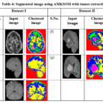Table 4: Segmented image using AMKSOM with tumor extraction     Click here to view Table

 

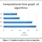Figure 2: Graphical analysis of processing time     Click here to view Figure

 

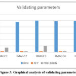Figure 3: Graphical analysis of validating parameters     Click here to view Figure

Conclusion

This research introduces a novel approach through the AMKSOM algorithm, which combines the strengths of both SOM and FKM to overcome the limitations of previous methods. From the experimental results, we have demonstrated that AMKSOM is highly effective in addressing the challenges of tumor detection in MRI images. Our algorithm significantly reduces the risk of manual errors made by physicians, which can delay diagnosis and treatment, ultimately helping patients receive timely intervention at earlier stages of tumor growth.

The results obtained using the proposed algorithm are promising and show substantial improvements in clustering accuracy, processing time, and overall efficiency. The success of this method opens the door for its application in other imaging modalities, such as PET scans and 3D imaging techniques, for the detection and diagnosis of other diseases. Further extensions of this approach could lead to more comprehensive diagnostic systems that can detect a wider range of medical conditions with higher precision.  

Acknowledgement

The authors sincerely thank Maharishi Markandeshwar (Deemed to be University), Mullana-Ambala, for their support and facilitation in carrying out this research work.

Funding Sources

The author(s) received no financial support for the research, authorship, and/or publication of this article.

Conflict of Interest

The author(s) do not have any conflict of interest.

Data Availability Statement

This statement does not apply to this article.

Ethics Statement

This research did not involve human participants, animal subjects, or any material that requires ethical approval.

Informed Consent Statement

This study did not involve human participants, and therefore, informed consent was not required.
Clinical Trial Registration

This research does not involve any clinical trials

Author Contributions

Karan Kumar: Analysis, Conceptualization & Methodology

Isha Suwalka: Analysis, Methodology, Writing – Manuscript.

Harishchander Anandaram: Methodology & Reviewing

Kapil Joshi: Visualization & Reviewing.

References

1. Bashab A, Ibrahim A O, Tarigo Hashem I A, Aggarwal K, Mukhlif F, Ghaleb F A, and Abdelmaboud A. Optimization Techniques in University Timetabling Problem: Constraints, Methodologies, Benchmarks, and Open Issues. Computers, Materials & Continua, 2023, 74, 3, 6461-6484.
   CrossRef
2. Dasgupta A, Gupta T, and Jalali R. Indian data on central nervous tumors: A summary of published work, South Asian J Cancer, 2016, 3, 147–153.
   CrossRef
3. Govindaraj V, Vishnuvarthanan A, Thiagarajan A, Kannan M and Murugan PR. Short Notes on Unsupervised Learning Method with Clustering Approach for Tumor Identification and Tissue Segmentation in Magnetic Resonance Brain Images, J Clin Exp Neuroimmunol, 2016, 1, 1-10.
4. Nandhagopal N. and Ganesh Automatic Detection of Brain Tumor through Magnetic Resonance Image. International Journal of Advanced Research in Computer and Communication Engineering, 2013, 2, 4, 1647-1651.
5. GuerroutH., Mahiou R. and Ait-Aoudia S. Medical Image Segmentation on a Cluster of PCs using Markov Random Fields, International Journal of New Computer Architectures and their Applications (IJNCAA). 2013, 3, 1, 35-44.
6. Ortiz A, Górriz JM, Ramírez J, Salas-Gonzalez D. and Llamas-Elvira, J.M. Two fully-unsupervised methods for MR brain image segmentation using SOM-based strategies”, Applied Soft Computing, 2013, 2668–2682.
   CrossRef
7. Aljahdali S. and Zanaty E. A. Automatic Fuzzy Algorithms for Reliable Image Segmentation. International Journal for Computers & Their Applications, 2012, 19, 3, 166-175.
8. Vasuda P. and Satheesh S. Improved Fuzzy C-Means Algorithm for MR Brain Image Segmentation. International Journal on Computer Science and Engineering, 2010;02(05): 1713-1715.
9. Abdi M.J., Hosseini S.M. and Rezghi M. A Novel Weighted Support Vector Machine Based on Particle Swarm Optimization for Gene Selection and Tumor Classification, Hindawi Publishing Corporation Computational and Mathematical Methods in Medicine, 2012; 7: 320698.
   CrossRef
10. Abdel-Maksoud , Elmogy M. and Al-Awadi R. Brain tumor segmentation based on hybrid clustering technique. Egyptian Informatics Journal, 2015;16: 71–81.
    CrossRef
11. Spanakis G. and Weiss G. AMSOM: Adaptive Moving Self-organizing Map for Clustering and Visualization, arXiv preprint arXiv:1605.06047, 2016.
    CrossRef
12. Dhanachandra N., Manglem K. and Chanu Y.J. Image Segmentation using K-means Clustering Algorithm and Subtractive Clustering Algorithm. Procedia Computer Science, Published by Elsevier B.V. under the Eleventh International Multi-Conference on Information Processing-2015; 54: 764 – 771.
    CrossRef
13. Roy S., Bhattacharyya D., Bandyopadhyay S.K. and Kim T.H. An iterative implementation of level set for precise segmentation of brain tissues and abnormality detection from MR images. IETE Journal of Research, 2017; 63(6): 769-783.
    CrossRef
14. Anwar A. and Iqbal A. Image Processing Technique for Brain Abnormality Detection, International Journal of Image Processing, 2013:7(1): 51-61.
15. Somasundaram K and Kalaiselvi T. Fully automatic brain extraction algorithm for axial T2-weighted magnetic resonance images. PubMed Comput Biol Med, 2012; 40: 811-822.
    CrossRef
16. Choksi K., Shah B. and Kale O. Intrusion Detection System using Self Organizing Map: A Survey, Journal of Engineering Research and Applications, 2014; 4(12): 11-16.
17. Abbood Z. A., Khaleel I., and Aggarwal K. Challenges and future directions for intrusion detection systems based on AutoML. Mesopotamian Journal of CyberSecurity, 2021;16-21.
    CrossRef
18. Alsharef A., Sonia, Arora M. and Aggarwal K. Predicting time-series data using linear and deep learning models—an experimental study. In Data, Engineering and Applications – Proceedings, 2022;505-516.
    CrossRef
19. Aggarwal K., Bhamrah M. S. and Ryait H. S. The identification of liver cirrhosis with modified LBP grayscaling and Otsu binarization. SpringerPlus, 2016; 5: 1-15.
    CrossRef
20. Rani P., Kumar R., Jain A., Lamba R., Sachdeva R.K., Kumar K. and Kumar, M. An Extensive Review of Machine Learning and Deep Learning Techniques on Heart Disease Classification and Prediction. Archives of Computational Methods in Engineering, 2024; 1-19.
    CrossRef
21. Rani P., Lamba R., Sachdeva R. K., Kumar K. and Iwendi C. A machine learning model for Alzheimer’s disease prediction. IET Cyber‐Physical Systems: Theory & Applications, 2024: 9(2): 125–134
    CrossRef

Abbreviations

AMSOM	Adaptive Moving Self-Organizing Map	MRF	Markov Random Fields
BMU	Best Matching Unit	MP	Maximum Probability
DE	Differential Entropy	MSE	Mean Square Error
DV	Differential Variance	PSNR	Peak Signal-To-Noise Ratio
DS	Dissimilarity	SOM	Self-Organizing Maps
FCM	Fuzzy C-Means	SA	Sum Average
FKM	Fuzzy K-Means	SE	Sum Entropy
GLCM	Gray-Level Co-Occurrence Matrix	SS	Sum Of Squares
ID	Inverse Difference	SV	Sum Variance
MRI	Magnetic Resonance Imaging