Swapna Katta¹, Prabhishek Singh², Deepak Garg¹ and Manoj Diwakar^3,4

¹School of Computer Science and Artificial Intelligence, SR University, Warangal, Telangana, India.

²School of Computer Science Engineering and Technology, Bennett University, Greater Noida, India,

³Department of CSE, Graphic Era Deemed to be University, Dehradun, Uttarakhand, India.

⁴Department of CSE, Department of CSE, Graphic Era Hill University, Dehradun, India.

Corresponding Author E-mail: prabhisheksingh1988@gmail.com

Abstract

The presence of gaussian noise commonly weakens the diagnostic precision of low-dose CT imaging. A novel CT image denoising technique that integrates the non-subsampled shearlet transform (NSST) with Bayesian thresholding, and incorporates a modern method noise Deep Convolutional neural network (DCNN) based post-processing operation on denoised images to strengthen low-dose CT imaging quality. The hybrid method commences with NSST and Bayesian thresholding to mitigate the initial noise while preserving crucial image features, such as corners and edges. The novel aspect of the proposed approach is its successive application of a DnCNN on initial denoised image, which learns and removes residual noise patterns from denoised images, thereby enhancing fine detail preservation. This dual-phase strategy addresses both noise suppression and image-detail preservation. The proposed technique is evaluated through the use of metrics, such as PSNR, SNR, SSIM, ED, and UIQI. The results demonstrate that the hybrid approach outperforms standard denoising techniques in preserving image quality and fine details.

Keywords

DnCNN; LDCT imaging; Gaussian noise; Method Noise; NSST

Copy the following to cite this article: Katta S, Singh P, Garg D, Diwakar M. A Hybrid Approach for CT Image Noise Reduction Combining Method Noise-CNN and Shearlet Transform. Biomed Pharmacol J 2024;17(3).

Copy the following to cite this URL: Katta S, Singh P, Garg D, Diwakar M. A Hybrid Approach for CT Image Noise Reduction Combining Method Noise-CNN and Shearlet Transform. Biomed Pharmacol J 2024;17(3). Available from: https://bit.ly/3BfPRum

Introduction

Medical imaging refers to the different imaging techniques used in modern hospitals and clinics for medical diagnosis. X-rays, CT imaging, ultrasound scans, magnetic-resonance imaging (MRI) techniques are used to scan within the body to assess the cause of disease and provide appropriate treatment for medical conditions. In CT imaging , X-ray radiation is directed at the patient’s body from multiple projections to scan bone fractures, organs, fat, and blood vessels. Although repeated scans in patients provide invaluable information for the clinical diagnosis of various diseases, there is a potential risk of  cancer threat^1,2. Hence, it is essential to minimize radiation exposure. Lowering radiation exposure improves noise, blur and other minute artifacts in tomographical images³. Low dose CT images exhibit noise due to electrical interference, quantum effects and mathematical computations. An effective denoising technique is required to explicitly reduce the noise and artifacts from distorted CT images ^4,5. CT image denoising techniques can be classified as classical CT image denoising, post-processing, and deep learning related methods.

Classical denoising techniques are classified as spatial and transform domain filtering methods. Spatial filtering methods manipulate the intensity values of the pixels directly based on spatial coordinates. Here, denoising is applied to the whole image. Spatial domain filtering methods,^6,7,8,9 make use of low-pass filtering, suppressing noise to some extent and resulting in blurry images, for example, wiener, mean, bilateral and nonlocal means (NLM) filtering show the correlation between pixel intensities in their neighboring pixels around a given pixel. This results in average smoothing, and a loss of sharp features in an image.

Transform domain filtering methods analyze images in terms of their frequency levels, for example., Discrete fourier transform, Discrete cosine transform, Wavelet, and Shearlet transform domain^10,11,12,13. In transform domain filtering, thresholding method is applied to denoise noisy CT images, and inverse transformation is used to reconstruct original images. Thresholding methods like SureShrink, VisuShrink, and BayesShrink. VisuShrink is a global thresholding method based on the pixel quantity in an image, where as SureShrink and BayesShrink based on each subband to evaluate the threshold values. The non-subsampled shearlet transform provides spatial localization and sparse representation of multiscale and multidirectional features to capture different directional features of an image to overcome the limitations such as isotropic features and the absence of multidirectionality of the wavelet transform. The shearlet transform is effectively used to capture and represent anisotropic features such as edges, corners, and fine details, and well-localized structures exhibit different features in different directions.

Unlike previous denoising techniques, post processing methods explicitly handle the reconstructed images in CT imaging, that is reconstruction without projectional data, which improves the performance of generalization. Traditional post-processing methods, Block-matching and 3D filtering (BM3D)¹⁴, adaptive nonlocal means (NLM)¹⁵, K means singular-valued decomposition (KSVD)¹⁶ methods effectively reduce noise and artifacts but the computational cost is high.

Hybrid methods are combinations of spatial and transform domain methods that provide improved image-denoising results, for example, denoising CT images through total variation using the shearlet domain¹⁷ with a multi-variate model, and method noise-based approach yield better results in suppressing noise, preserving the edges and structural details. The detection of noisy COVID-19 (SARS-CoV-2) virus on LDCT imaging using the nonlocal means filter in conjunction with method noise yields improved SSIM results compared to other existing methods¹⁸, for example, nonlocal means¹⁹ , total-variation methods²⁰ using wavelets, to reduce noise while preserving image features in detail. However, images suffer from noise and artifacts owing to poor directionality, shift sensitivity, and a limited ability to capture directional information.

Recently, deep learning  techniques have played a crucial role in image denoising.The progress in CNN-based methods^21,22  has improved in CT image denoising in LDCT imaging. The deep denoising convolutional neural network with residual learning strategy (REDCNN) is a CNN architecture used in image denoising that includes residual mapping trained deeper networks to resolve the vanishing-gradient problem and allows deeper networks to be trained easily. The efficiency of the deep CNN differs at different CT radiation dose levels. For example, the Wasserstein distance-based generative adversarial network (W-GAN) provides superior GAN performance, and perceptual loss evaluates perceptual features with filtered output at ground truth level to maintain critical information and effectively reduce noise in CT images²³. Currently, transformer models play a significant role in image- processing. The Transformer model is a (DL) deep learning architecture, which is a self-attention mechanism that captures long-range dependencies between input and output tokens²⁴. A vision transformer (ViT) is a kind of neural-network framework, especially applied in domains like image recognition, recognition, and segmentation. Transformer-based Encoder-decoder Dilation network (TED) effectively preserves the structure and fine details while denoising images²⁵.

Problem Statement

CT imaging is essential for accurate healthcare diagnostics because it provides precise images for the detection of  health conditions. However, the existence of Gaussian noise in CT images significantly diminishes their quality, contributing to potential challenges in disease prediction and identification. This study aims to address the significant need for effective noise suppression method to improve CT image quality, thereby improving diagnostic precision and patient clinical judgement.

Major Contribution

The study presents a novel CT imaging denoising technique that combines method noise-based CNN with a non-subsampled shearlet transform to effectively mitigate Gaussian noise .The proposed technique improves noise suppression while retaining crucial image features by leveraging the multi-scale and multi-directional analysis of the shearlet transform. Additionally, the method noise-based CNN method intends to reduce residual noise patterns in denoised CT images. This hybrid strategy significantly improves image quality and diagnostic accuracy, providing an effective solution to noise-related challenges in LDCT imaging.

The rest of this paper is presented as follows. Section 2 introduces a brief literature review of CT image-denoising approaches. Section 3 outlines the major concepts of shearlet transform and DnCNN architecture. Section 4 discusses the proposed hybrid algorithm for CT image denoising with a method noise-based CNN method using a shearlet transform. The findings from the experiments and a comparison with various existing denoising methods are shown in Section 5. Finally, the conclusions and proposed future studies are presented in Section 6.

Literature Review

Clinical imaging plays a major role in diagnostic decision making using different modalities, to improve the accuracy of clinical diagnosis of the internal human body. In,²⁶  Abhisheka proposed that the prominent medical imaging modalities include X-radiation, CT scan, MRI, Positron-Emission Tomographical (PET) imaging, and Ultrasound scans. These modalities effectively visualize a detailed image of inside the human body. For example, X-rays can be used to identify bone fractures, dislocations. Unlike X-ray, a CT scan provides a fast, more detailed image for medical diagnosis. CT scan is used to detect organ abnormalities, blood clots, subtle bone fractures, and internal bleeding. MRI scans provide highly detailed images of soft tissues. Ultrasound, or sonography, exploits  high frequency  sound waves to provide detailed imaging of human body, detect problems in the liver, kidney, heart, blood vessels, valvular regurgitation, and abdominal aorta etc. PET scans are used for detecting organ abnormalities, including soft tissue-related issues such as finding tumors, neurological (brain) diseases, cardiovascular (heart) diseases. These medical image modalities are used by healthcare professionals to diagnose various medical conditions in a timely, accurate, and non-invasive manner, thereby improving patient outcomes.

The proposed literature review primarily concentrates on CT imaging using various deep learning approaches. In,²⁷ Sehgal proposed novel CT image denoising algorithm, Political-Taylor Anti-coronavirus Optimization (PT-ACVO) combines deep learning and advanced optimization techniques to mitigate noise and enhance image qualities effectively. The method detects noisy pixels in images using a Deep Residual  network (DRN) and reconstructs them using the Political Taylor-Anti-Coronavirus Optimization (Political Taylor -ACVO) algorithm and image-enhancement is achieved through Vectorial-Total-Variation approach. Image denoising was performed using Discrete Wavelet transform and NLM filtering, followed by image fusion to obtain final denoised image. However, the DRN and the Political-Taylor-ACVO Optimization algorithm might cause higher computational complexity and there is a requirement for extensive parameter-tuning.

The evolution of Deep learning methods has emerged as a rapid progress in CT image denoising²⁸. To improve the quality of LDCT imaging,²⁹ Zhang proposed an innovative denoising method using U-net and multi-attention mechanisms for effective feature extraction. This includes three attention modules. The local attention module provides localized surrounding pixel feature extraction based on feature mapping. The multi feature and channel-attention-module automatically acquire, extract, suppress noise, and contribute different weights to the existing feature-map based on different tasks. The hierarchical identification module enabled a deeper CNN for a substantial amount of feature extraction. Additionally, a study suggests that the enhanced learning-module increases the network depth by stacking a multi-layered CNN, activation layer and batch-normalization (BN) enabling the learning and maintenance of  detailed image information. The Experimental quantitative analysis results show that the module effectively suppressed noise.

In,³⁰ Huang proposed a deep cascade residual network (DCRN) that offers promising denoising results, combining attention mechanisms to enhance model performance, a hybrid loss function to provide better generalization ability of the model, and iterative refinement to iteratively refine the denoised image to obtain a better-quality image. In,³¹ Selig proposed a Dilated Residual U-Net (DRU-Net) for better LDCT image reconstruction and image enhancement to enhance image quality and performance. This involves two-stage process: Initially, filtered-back projection (FBP) was performed to improve image reconstruction. DRU-Net is pre-trained for denoising natural grayscale images, and mapping low-dose filtered back projection is applied to the reconstructed images to enhance the CT images. DRU-Net is fine-tuned and performs downstream image enhancement  by leveraging LDCT imaging  and appropriate normal-dose computed tomographical (NDCT) images. This method secured the topmost ranking in the low dose parallel beam CT-challenge (LoDoPaB), was computationally more efficient than Institute of Technology Network (ItNet), and increased the SSIM metric value. Here, the U-Net model was pretrained only for Gaussian denoising. If the pre-trained task and target CT image denoising differ, affects the performance of the model.

In,³² Song introduced a NeXtResUNet-CNN for industrial CT image denoising. It includes industrial CT image systems that operate on diverse energies and significantly affect distinct spatial resolutions. The proposed algorithm initiates an image fusion network that combines Con-vNeXt, ResNet, and U-Net, is assigned to a self-generated industrial tomographic denoising dataset. NeXtResUnet simulates a transformer model to acquire global features, and ResNet is used to extract the image details. CT-image noise reduction can be accomplished by downsampling the CNN. This results in an improved Peak signal-to-noise ratio (PSNR) and image-denoising, image segmentation, and contrast normalization. The NeXtResUNet network structure is concise and expandable, making it applicable to image denoising and image vision-based tasks, like CT image super-resolution and auto-segmentation involving industrial CT data.

In,³³ Byeon proposed the use of a lightweight Deep CNN with multi-directional fuzzy non subsampled shearlet transformation (FNSST) for better image decomposition and suppression of noisy patterns and artifacts in LDCT imaging. FNSST is a multi-scale and multi-directional localization technique used for the decomposition of low and normal dose images to produce high and low-resolutional subimages. High-resolutional subimages with varying noise levels in a fuzzy setting and other artifacts were given as input to the CNN to establish an association between the LDCT high-resolution subimages and  the residual subimages generated throughout the training process. FNSST-CNN discriminates low and high-frequency subimages while testing process to suppress noise and other relevant artifacts. In LDCT imaging, FNSST-CNN effectively reduces noisy patterns while preserving the edges and structural features. The main limitation is that the cost of implementing fuzzy-based methods is high.

In,³⁴ Li proposed a multistage noise reduction framework for LDCT images. The framework was mainly trained using un-paired data. The (PCCNN) Progressive-Cyclical-CNN  performs latent -space utilization from CT images to suppress noisy areas and other artifacts. PCCNN, a multistage denoising framework, suggests a noise transfer model that enables the transfer of noise from low-dose to normal dose CT images. The PCCNN also has a progressive module that includes a multi-stage wavelet transform to extract high frequency coefficients to reduce noisy coefficients and preserve contours of the image. The main constraint is that there is a need for pairs of perfectly matched low and normal-dose images to elevate model performance.

In,³⁵ Çalişkan introduced, effective method for identifying and handling noisy pixels in 2D images using  to enhance the quality of CT images, specifically focusing on accurate detection of noisy pixels in  2 Dimensional CT images using hidden resource decomposition approach. The hidden resource decomposition approach with extreme learning Machines (ELM) to improve efficiency in training and high learning speed suitable for handling large volumes of the CT images to preserve critical structural information in detail. The ELM method markedly improved noise suppression and imaging quality, attaining peak performance with 250 hidden layer neurons. he ELM method significantly reduced mean- squared-error (MSE) and peak-signal-to-noise ratio (PSNR).The incorporation of hidden resource decomposition with ELM may result in complexity in implementation.In,³⁶ Çalişkan suggested, deep learning-driven hybrid approach to categorize seven mineral types, with precision, employing refined feature selection and the complement rule for clustering. The method utilizes deep learning models for feature-extraction and applied metaheuristic optimization to identify key features, and complement rule for grouping ineffective features for achieving exceptional classification precision. The image denoising can be obtained using metaheuristic optimization algorithm due to their capability to explore vast and complex search spaces.

Major Concepts

The following section presents some essential concepts that were exploited to implement the proposed methodology.

Non-subsampled Shearlet Transform

The NSST transform is constitutes an extended variant form of wavelet transformation and is a mathematical tool,³⁷ used in image processing, particularly for image denoising and feature extraction. The nonsubsampled shearlet transform is a  multi-directional, multi-dimensional, shift-invariant, and well-localized analysis that combines multiscale and directional analysis separately. NSST coefficients are related to sparse and capture the mathematical and geometric properties of an image. NSST is depicted in conjunction with Nonsubsampled-Laplacian pyramid (NS-LP) and shearing-filters. Initially, (NSLP) is used to analyze the images into different low (approximation) and high (detail) frequency components, and directional filtering helps to generate various subbands and extract shearlet components. The shear matrix accomplishes directional filtering and provides an analysis across various directions.

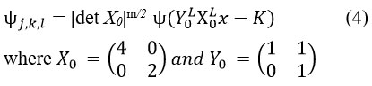
For image data with dimensions of n=2, and for j>0, k ∈ R, l ∈ R²

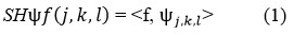
Where ψf(j, k, l) are called shearlets. Here, j > 0, k ∈ R, l ∈ R², the shearlets are evaluated as:

The anisotropic-dilation is represented as:

where j>0, manages the shearlet’s scale, and provides the frequency to obtain finer scales. The shearing transformation matrix is obtained as follows:

The shearing matrix manages only the shearlet direction.

Hence, the shearlet transform is determined by the three variables, includes scale j, orientation k and location l.

Each f ∈ L² (R²)is restored using:

The Discrete shearlet transform is used to represent multi-dimensional functions. Here j= 2^-2m ,k=-L with m, l=k∈Z² and L ∈ Z.

The Discrete shearlet transformation can be denoted as:

From each function f ∈ L² (R²),the given method is reconstructed using the characteristics of as described below:

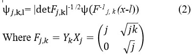
The fundamental framework of DnCNN is depicted in Fig. 1.

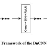Figure 1: Framework of the DnCNN network   Click here to view Figure

 

Architecture of DnCNN

The DnCNN architecture,²⁸ has been extensively utilized in image restoration and artifact removal. DnCNN is a popular neural network denoising framework that is intended to denoise additive white Gaussian noise, image restoration, single image super-resolution, and deblocking JPEG images. For a given noisy input image, the noise observation is denoted as x = y + v, and the discriminative model for denoising attempts to acquire the mapping-function, F(x) = y. The DnCNN approach leverages the residuals or skip connection learning process to train the residual transformation R(x) = v; subsequently, y = x – R(x), and DnCNN applies the loss function (l) to enhance model parameters that are R (∂) specific to the DnCNN framework.

The Loss function is calculated as the average mean-squared error among the residual and the predicted image based on noisy images.

The training process of the DnCNN was performed using a loss function.

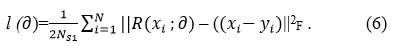
where,

∂ represents trainable parameters of the DnCNN network.

N represents the pairs of clean and distorted training image patches.

The architecture of the DnCNN was accustomed to reduce boundary artifacts. It includes

Deep Architecture

DnCNN architecture with depth D, includes 3 types of layers.

Layer 1

Convolutional_layers + ReLu (Rectified Linear Unit) activation function, including 64 filters with each aspect of existed dimensions [3 × 3 × c] (total channels) to generate 64 feature representations and Rectified Liner Units. Here, non linearity is obtained by ReLu ((max (0,.)). Here, the channel quantity for grayscale image is 1; The number-of-channels for a color image is 3 (R-red, G-green, B-blue).

Layer 2

Convolutional_layer + ReLu + Batch normalization (BN) through the addition of 64 convolutional_filters, the size of each dimension is  3 × 3 × 64, batch normalization was performed  between each aspect of the convolutional_layer and the (ReLu ) activation function, and the depth of the layers was 2 ~ (D – 1).

Layer 3

The convolutional_layer is mainly applied for image restoration via 64 filters of size 3 × 3 × 64.

Reducing Boundary Artifacts

In general, core vision techniques require the size of resulting image to be consistent with the given input image. Here, DnCNN applies simple-zero padding and  does not exhibit any artifacts. DnCNN directly pads the zeroes before convolution; thus, each feature mapping relating to existing middle layers exhibit a size equivalent to that of the specified image.

The main contribution of DnCNN in noise reduction approach is that, it effectively utilizes the residual network strategy and batch normalization process to expedite the training and regularize the learning problem. The image Denoising approach is represented as a Discriminative-learning challenge  to separate distortion from latent images.

Method noise refers to residual noise or artifacts introduced by the denoising algorithm used in image processing. The residual noise retains pixel information in the image after applying a noise suppression or denoising algorithm. This shows the discrepancy among a noisy input and a (filtered) denoised image.

Method noise = noisy input image – denoised (processed) image.

Method noise was applied to assess the effectiveness of the denoising techniques while preserving image structure and fine details.

Proposed Methodology

In this portion, firstly describe the flowchart and proposed methodology in detail.

Mathematically, image denoising can be represented as:

 Y1 (i, j) = X1 (i, j) + n1(i, j).

where X1 (i, j) denotes a clean image, Y1 (i, j) denotes a noisy or distorted  CT image, and n1 is supposed to be (AWGN) Additive-White-Gaussian-Noise in conjunction with a standard deviation (σ), and (i, j) represents pixel’s locations in an image.

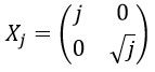
The comprehensive summary of the suggested  approach is depicted in Fig. 2. The proposed hybrid approach combining the preprocessing approach of NSST and postprocessing approach of method noise with CNN to achieve superior denoising results, i.e., effectively combining the structural features of NSST, the statistical features of Bayesian thresholding,³⁸ and the learning capability of method noise-based CNN ,³⁹ will further enhance the image denoising approach.

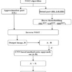Figure 2: Flowchart of proposed CT image denoising using NSST with method noise-based CNN.   Click here to view Figure

 

Proposed Algorithm

Input: A Pre-processed, noisy CT image A_i,j.

Output: Final denoised CT image A”_i,j.

Step 1: Perform NSST transform to decompose gaussian noisy input CT image A_i,j to acquire low- frequency components NSST_A^l and high-frequency components NSST_A^l (HL ^new, LH ^new and HH ^new).

Step 2: Implement CT image denoising using the following steps:

Evaluate noise variability.

Determine thresholding value.

Implement empirical Bayesian thresholding method on noisy  coefficients to obtain thresholded NSST coefficients.

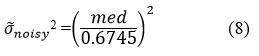
Evaluate Noise Variance

Estimate noise variance σ ̃noisy from noisy shearlet coefficients using robust median estimation ⁴⁰ of CT image noise level in (HH) high-high shearlet diagonal coefficients.

Estimate the noise standard deviation σ ̃noisy

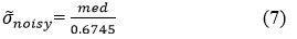
med= median (|c_k (:)|), ∈HH subbands

where

c_k represents set of high frequency (HH) coefficients of NSST decomposition of noisy CT image.

med represents median absolute deviation  of all coefficients.

The constant 0.6745 is used for robust estimation of the noise level.

Calculate noise variance σ ̃noisy²

Implement Bayesian Thresholding Process

The threshold value is calculated for retaining the image’s intricate details of an image and perform noise suppression effectively.

The threshold value is selected as:

where,

⅄ ̃_i,j denotes the threshold value used for empirical Bayes thresholding.

σ ̃noisy²  denotes the estimated noise variation.

∅ⁿ (A_i,j) denotes the amount of elements of image Ai,j.

log signifies the natural logarithm function.

Perform thresholding of coefficients t_k using empirical Bayes thresholding.

Bayesian soft thresholding process:

For each coefficient|Ai,j|, find the absolute value of Ai,j.

Compute the sign of the coefficients.

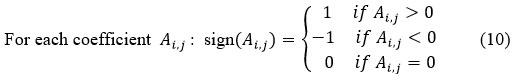
Apply Bayesian soft thresholding approach for each coefficient, is described as:

This function works as follows for thresholding:

 If |Ai,j| is  less than or equal to (<=), the given thresholding A ̃ i,j is set to 0. This procedure effectively removes small coefficients assumed to be dominated by gaussian noise. Then replace the original noisy coefficients Ai,j with thresholded coefficients t_k

Step 3: Perform inverse NSST transform on thresholded NSST_A^h  coefficients (HL^new, LH ^new and HH ^new) to reconstruct the semi denoised CT image, B_i,j.

Calculate the residual image A’i,j.

Here A’i,j represents the discrepancy between a noisy image Ai,j and its reconstructed semi denoised image counterpart B_i,j.

When A’i,j approaches 0, the noise in the original signal is successfully eliminated through denoising. A’i,j is residual image that also has some noisy coefficients that affect the quality of image.

Step 4: Calculate C’i,j by applying method noise CNN on residual image A’ i.e., DnCNN on (A’i,j).

Step 5: calculate final denoised image

By combining inverse thresholded NSST coefficients (Bi,j) with the denoised method noise-based CNN on the residual image (Ci,j) to get the final denoised image (A’’i,j).

A Brief Explanation of Proposed Methodology

During the experiments , noisy CT images are commonly contaminated by Gaussian noise, The hybrid approach, non-subsampled shearlet transform is applied for decomposition of noisy image into an approximation  (LL ^new) and detail part  (LH ^new, HL ^new and HH ^new). The (approximation) high frequency components are further decomposed into multidirectional subbands to represent image features in a detailed manner. The noise variance was estimated in high frequency components using the median-absolute-deviation (MAD).The Bayesian thresholding function, which selects all noisy NSST coefficients, then calculates optimal threshold values to obtain the denoised coefficients. The inverse NSST transform is used to reconstruct denoised CT images from high frequency thresholded NSST coefficients, resulting in a denoised CT image. The denoised image, that is, the reconstructed image, preserves fine details but  retains some residual noise. To solve this problem, calculated the method noise to visualize the discrepancies among  the noisy and denoised NSST coefficients. Here, the method noise process was applied to capture residuals or any distortions introduced during the CT image denoising process. The deep CNN,²⁸ network architecture is applied to method noise to learn complex noise patterns in order to capture intricate details effectively and reduce noise components. Finally, residual learning denoised image was combined with the NSST high frequency thresholded denoised image to acquire the final denoised CT-image. The final restored image preserves fine details and structural information while simultaneously removing noise and other artifacts.

Results and Discussion

The exploratory evaluation is carried out on noisy grayscale CT images with pixel’s size 512×512.  Initially, CT scan test images are obtained from “large COVID-19 CT-scan slice dataset” to determine the efficacy of the suggested denoising method. The Noise-free or clean CT images are required as a reference image to analyse the denoising method’s performance. Fig. 3. is considered as CT images 1, 2,3, and 4 respectively. Fig. 4. depicts the addition of additive gaussian  with a noise variance of 10. To test the experimental results, Additive-white-gaussian-noise is added at different noise levels(𝜎 = 5, 10, 15, 20) to analyze the effectiveness of various denoising techniques and assess the qualitative performance of noisy CT images.

Quantitative Evaluation Metrics

The qualitative result analysis of the suggested methodology uses diverse quality factors , i.e., PSNR, SNR, SSIM, ED, and UIQI,^10,41.

PSNR (Peak Signal-to-Noise ratio) is used to assess the quality of restored images relative to the original images. PSNR evaluates the ratio between the given maximum signal strength and the power of distorted noise, i.e., the difference between the clean image and filtered image. For the input CT image X and the denoised CT image Y.

PSNR is denoted as

Where MSE represents the mean-square-error between the original image and the denoised CT image.

X (i, j) depicts the clean CT image.

Y (i, j) depicts the filtered CT image.

m x n represents the pixel’s size of clean CT image and a denoised CT image.

(SNR) Signal-to-Noise ratio is a qualitative metric to measure and quantify the desired signal strength related to the distortion or noise level. It is measured in the form of decibels, and it is also used to analyze the image quality.

SSIM (Structural-Similarity-Index-Measure) is a metric serves as a measure to evaluate the similarity among two images. It is mainly relying on three parameters: luminance, contrast, and structural features, and the SSIM values vary between -1 and 1, where 1 denotes absolute similarity and -1 denotes discrepancy between two images.

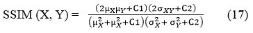
X represents clean CT image.

Y represents denoised or filtered CT image.

µ_X and µ_Y are denoted as the local means, σ_X, σ_Y are denoted as standard deviations, and σ_XY is image’s covariance of  X and Y Here, C1=(k1D)², C2= (k2D)² are constant values to stabilize division with zeros, where D is the variation in pixel values between 2^{bits-per-pixel} -1 and 1. Here, k1= 0.01 & k2 = 0.03.

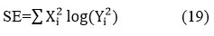
The Entropy Difference is the statistical measure of randomness present in an image suitable for analyzing the texture of the given source images. Shannon entropy is estimated between the clean image (X_i) and the denoised-CT image (Y_i). The dissimilarity in the mean value is denoted as ED.

ED is computed as:

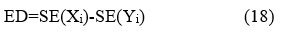
Where, SE denotes Shannon Entropy.

Shannon Entropy is computed as:

UIQI (Universal-Image-Quality-Index) is a benchmark used to determine the quality of a denoised CT image and its corresponding reference image.

The UIQI between two images original image distorted image is defined as:

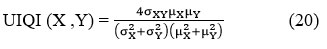
μ_X μ_Y represents the average values of the given CT images X and Y.

σ_x² and σ_y²denotes the variances of X and Y.

σ_XY represents the covariance of the images X and Y.

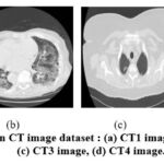Figure 3: Clean CT image dataset : (a) CT1 image, (b) CT2 image, (c) CT3 image, (d) CT4 image.   Click here to view Figure

 

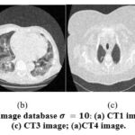Figure 4: Noisy CT image database (a) CT1 image; (b) CT2 image;  (c) CT3 image; (a)CT4 image.   Click here to view Figure

 

Table 1: PSNR Comparison for the proposed methodology with wiener, median, bilateral, DWT, curvelet transform, contourlet transform, and DnCNN for CT1, CT2, CT3, and CT4 images at various gaussian noise variances (𝜎=5, 10, 15, 20 of noise intensity).

CT Image	𝜎	PSNR				CT Image	PSNR
		5	10	15	20		5	10	15	20
CT 1	Wiener filter9	26.9227	21.0561	17.1016	15.9510	CT 2	28.8351	22.3409	20.0957	18.0717
512×512	Median filter6	25.4818	21.2815	18.0291	16.1741	512×512	26.8228	22.6641	19.3134	17.7229
	Bilateral filter7	25.8456	20.9348	18.3621	15.5553		28.2931	22.3078	19.6007	17.4489
	NSST with Bivariate17	35.0639	29.4426	26.1123	23.7630		34.9416	29.2023	25.8483	23.5604
	DWT11	36.1510	31.7197	28.9528	27.1211		36.8484	32.4378	29.6757	27.8361
	Curvelet transform12	24.7381	17.8315	15.2633	15.2232		24.4989	17.8109	15.2434	15.3776
	Contourlet transform13	31.1441	28.4641	27.7560	27.4756		31.9356	29.3965	28.6934	28.5351
	DnCNN28	26.9654	21.3395	17.8176	16.1083		27.1848	23.4148	19.8904	17.8606
	Proposed method	38.6875	35.4432	33.5507	32.0938		39.3028	35.7841	33.6865	32.2141
CT 3	Wiener filter9	27.2958	21.5341	18.9843	15.5837	CT 4	30.4803	24.1262	20.8647	19.7389
512×512	Median filter6	27.6440	20.3498	17.9301	16.7986	512×512	29.9581	24.2495	20.9963	19.8384
	Bilateral filter7	27.4662	21.0894	18.3180	16.2724		31.6511	24.4505	20.8721	19.4807
	NSST with Bivariate17	34.6530	28.8408	25.4758	23.1329		34.5294	28.9670	25.8372	23.6112
	DWT11	37.7380	32.8812	30.1778	27.9877		35.9373	31.3968	28.6151	26.5497
	Curvelet transform12	24.1199	17.7353	15.3748	15.5832		24.6752	18.2605	15.7387	15.7257
	Contourlet transform13	31.2001	28.7470	28.1473	27.9475		32.1699	30.3563	30.0802	30.2322
	DnCNN28	25.5178	21.4493	19.0634	16.3844		30.2987	25.0755	22.3263	19.9453
	Proposed method	40.0415	37.0541	35.2108	33.7444		38.7044	35.1286	33.1462	31.7048

Table 2: SNR comparison for the suggested approach with wiener, median, bilateral, DWT, curvelet transform, contourlet transform, and DnCNN for CT1, CT2, CT3, and CT4 images at various gaussian noise variances (𝜎=5, 10, 15, 20 of noise intensity).

CT Image	𝜎	SNR				CT Image	SNR
		5	10	15	20		5	10	15	20
CT 1	Wiener filter 9	23.1806	17.3140	13.3595	12.2089	CT 2	24.3356	17.8414	15.5962	13.5722
512×512	Median filter6	21.7397	17.5394	14.2870	12.4320	512×512	22.3233	18.1646	14.8139	13.2234
	Bilateral filter7	22.1035	17.1927	14.6200	11.8132		23.7936	17.8083	15.1012	12.9494
	NSST with Bivariate17	31.3218	25.7005	22.3702	20.0209		30.4421	24.7028	21.3488	19.0609
	DWT11	32.4093	27.9826	25.2195	23.3900		32.3488	27.9392	25.1814	23.3493
	Curvelet transform12	20.8339	13.7838	11.1153	10.9738		19.9783	13.2432	10.6259	10.6641
	Contourlet transform13	21.0065	14.0935	11.5272	11.3866		19.9740	13.2892	10.8254	10.8066
	DnCNN28	23.2233	17.5974	14.0755	12.3663		22.6853	18.9153	15.3909	13.3611
	Proposed method	34.9454	31.7011	29.8086	28.3517		34.8033	31.2846	29.1870	27.7154
CT 3	Wiener filter9	24.3152	18.5534	16.0036	12.6031	CT 4	24.7123	18.3583	15.0967	13.9709
512×512	Median filter6	24.6634	17.3691	14.9494	13.8179	512×512	24.1901	18.4815	15.2284	14.0705
	Bilateral filter7	24.4855	18.1087	15.3373	13.2917		25.8831	18.6825	15.1041	13.7127
	NSST with Bivariate17	31.6724	25.8601	22.4952	25.1522		28.7614	23.1990	20.0692	17.8432
	DWT11	34.7583	29.9035	27.2033	25.0127		30.1727	25.6366	22.8592	20.7994
	Curvelet transform12	21.1356	14.6744	12.1857	12.2720		18.9421	12.6007	10.0722	09.9956
	Contourlet transform13	21.0577	14.7171	12.4321	12.5608		18.8854	12.5286	09.9644	09.9185
	DnCNN28	22.5371	18.4687	16.0827	14.4038		24.5307	19.3075	16.5583	14.1773
	Proposed method	37.0609	34.0742	32.2301	30.7637		32.9364	29.6594	27.3780	25.9118

Table 3: SSIM comparison for the proposed ensembled approach with wiener, median, bilateral, DWT, curvelet transform, contourlet transform, and DnCNN for CT1, CT2, CT3, and CT4 images at various gaussian noise variances (𝜎=5, 10, 15, 20 of noise intensity).

CT Image	𝜎	SNR				CT Image	SNR
		5	10	15	20		5	10	15	20
CT 1	Wiener filter 9	23.1806	17.3140	13.3595	12.2089	CT 2	24.3356	17.8414	15.5962	13.5722
512×512	Median filter6	21.7397	17.5394	14.2870	12.4320	512×512	22.3233	18.1646	14.8139	13.2234
	Bilateral filter7	22.1035	17.1927	14.6200	11.8132		23.7936	17.8083	15.1012	12.9494
	NSST with Bivariate17	31.3218	25.7005	22.3702	20.0209		30.4421	24.7028	21.3488	19.0609
	DWT11	32.4093	27.9826	25.2195	23.3900		32.3488	27.9392	25.1814	23.3493
	Curvelet transform12	20.8339	13.7838	11.1153	10.9738		19.9783	13.2432	10.6259	10.6641
	Contourlet transform13	21.0065	14.0935	11.5272	11.3866		19.9740	13.2892	10.8254	10.8066
	DnCNN28	23.2233	17.5974	14.0755	12.3663		22.6853	18.9153	15.3909	13.3611
	Proposed method	34.9454	31.7011	29.8086	28.3517		34.8033	31.2846	29.1870	27.7154
CT 3	Wiener filter9	24.3152	18.5534	16.0036	12.6031	CT 4	24.7123	18.3583	15.0967	13.9709
512×512	Median filter6	24.6634	17.3691	14.9494	13.8179	512×512	24.1901	18.4815	15.2284	14.0705
	Bilateral filter7	24.4855	18.1087	15.3373	13.2917		25.8831	18.6825	15.1041	13.7127
	NSST with Bivariate17	31.6724	25.8601	22.4952	25.1522		28.7614	23.1990	20.0692	17.8432
	DWT11	34.7583	29.9035	27.2033	25.0127		30.1727	25.6366	22.8592	20.7994
	Curvelet transform12	21.1356	14.6744	12.1857	12.2720		18.9421	12.6007	10.0722	09.9956
	Contourlet transform13	21.0577	14.7171	12.4321	12.5608		18.8854	12.5286	09.9644	09.9185
	DnCNN28	22.5371	18.4687	16.0827	14.4038		24.5307	19.3075	16.5583	14.1773
	Proposed method	37.0609	34.0742	32.2301	30.7637		32.9364	29.6594	27.3780	25.9118

Table 4: ED Comparison for the proposed approach with wiener, median, bilateral, DWT, curvelet transform, contourlet transform, and DnCNN for CT1, CT2, CT3, and CT4 images at various gaussian noise variances (𝜎=5, 10, 15, 20 of noise intensity).

CT Image	𝜎	ED				CT Image	ED
		5	10	15	20		5	10	15	20
CT 1	Wiener filter9	0.2614	0.4414	0.5418	0.6709	CT 2	0.2177	0.3527	0.4904	0.5725
512×512	Median filter6	0.2170	0.4034	0.5029	0.5559	512×512	0.2219	0.3135	0.3555	0.4014
	Bilateral filter7	0.1795	0.4045	0.5949	0.7027		0.1673	0.3201	0.4543	0.5704
	NSST with Bivariate17	0.4774	0.7059	0.8858	1.0016		0.5220	0.7635	0.9367	1.0175
	DWT11	0.1864	0.0496	0.0314	0.0524		0.7585	0.6040	0.5585	0.4996
	Curvelet transform12	0.5713	0.5397	0.5113	0.5491		0.5713	0.5397	0.5113	0.5491
	Contourlet transform13	0.5716	0.5356	0.5147	0.5532		0.0596	0.0004	0.0272	0.0219
	DnCNN28	0.2900	0.1760	0.1220	0.0996		0.2331	0.1782	0.1261	0.1137
	Proposed method	0.0383	0.0583	0.0719	0.0841		0.0330	0.0550	0.0699	0.0793
CT 3	Wiener filter9	0.0944	0.2976	0.4661	0.4913	CT 4	0.0019	0.0415	0.0594	0.0611
512×512	Median filter6	0.1303	0.2915	0.3970	0.4959	512×512	0.0165	0.1158	0.1584	0.1983
	Bilateral filter7	0.0648	0.2603	0.4550	0.6012		0.0449	0.0429	0.0566	0.1164
	NSST with Bivariate17	0.5307	0.8390	1.0659	1.2341		0.3086	0.4871	0.5824	0.6565
	DWT11	0.0734	0.0207	0.0020	0.0052		0.0342	0.0760	0.1391	0.2021
	Curvelet transform12	0.2521	0.2080	0.2045	0.2320		0.0490	0.1310	0.1386	0.0825
	Contourlet transform13	0.2514	0.2189	0.2108	0.2303		0.0511	0.1296	0.1394	0.0881
	DnCNN28	0.0544	0.0314	0.0292	0.0307		0.0521	0.1397	0.1617	0.1828
	Proposed method	0.0361	0.0544	0.0772	0.0771		0.0204	0.0360	0.0484	0.0587

 

Table 5: UIQI Comparison for the proposed method with comparison of UIQI values with wiener, median, bilateral, DWT, curvelet transform, contourlet transform, and DnCNN for CT1, CT2, CT3, and CT4 images at various gaussian noise variances (𝜎=5, 10, 15, 20 of noise intensity).

CT Image	𝜎	UIQI				CT Image	UIQI
		5	10	15	20		5	10	15	20
CT 1	Wiener filter9	0.9945	0.9776	0.9412	0.9209	CT 2	0.9958	0.9803	0.9655	0.9430
512×512	Median filter6	0.9922	0.9792	0.9543	0.9277	512×512	0.9935	0.9824	0.9602	0.9408
	Bilateral filter7	0.9930	0.9700	0.9567	0.9130		0.9953	0.9802	0.9613	0.9339
	NSST with Bivariate17	0.9989	0.9959	0.9910	0.9845		0.9983	0.9949	0.9890	0.9812
	DWT11	0.9991	0.9976	0.9955	0.9931		0.9991	0.9976	0.9955	0.9932
	Curvelet transform12	0.9874	0.9363	0.8822	0.8774		0.9874	0.9363	0.8822	0.8774
	Contourlet transform13	0.9874	0.9364	0.8824	0.8746		0.9848	0.9275	0.8696	0.8644
	DnCNN28	0.9947	0.9800	0.9525	0.9272		0.9940	0.9854	0.9656	0.9431
	Proposed method	0.9995	0.9989	0.9984	0.9977		0.9995	0.9989	0.9982	0.9975
CT 3	Wiener filter9	0.9955	0.9824	0.9667	0.9212	CT 4	0.9963	0.9834	0.9631	0.9510
512×512	Median filter6	0.9960	0.9779	0.9600	0.9462	512×512	0.9958	0.9839	0.9645	0.9527
	Bilateral filter7	0.9957	0.9807	0.9614	0.9348		0.9972	0.9847	0.9633	0.9479
	NSST with Bivariate17	0.9979	0.9917	0.9820	0.9693		0.9985	0.9946	0.9888	0.9812
	DWT11	0.9989	0.9967	0.9939	0.9899		0.9989	0.9969	0.9941	0.9906
	Curvelet transform12	0.9751	0.8941	0.8200	0.8228		0.9853	0.9346	0.8800	0.8759
	Contourlet transform 3	0.9747	0.8934	0.8291	0.8207		0.9853	0.9350	0.8798	0.8747
	DnCNN28	0.9936	0.9833	0.9703	0.9429		0.9962	0.9869	0.9744	0.9540
	Proposed method	0.9993	0.9989	0.9981	0.9973		0.9994	0.9986	0.9979	0.9971

 

Visual Evaluation of the Experimental Results with Additive White Gaussian Noise

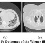Figure 5: Outcomes of the Wiener filter [9].   Click here to view Figure

 

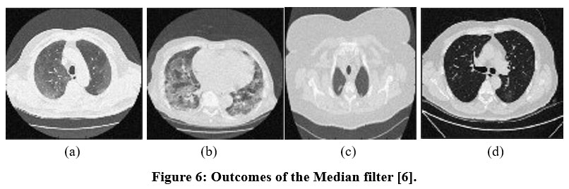Figure 6: Outcomes of the Median filter [6].   Click here to view Figure

 

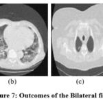Figure 7: Outcomes of the Bilateral filter [7].   Click here to view Figure

 

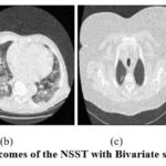Figure 8: Outcomes of the NSST with Bivariate shrinkage [17].   Click here to view Figure

 

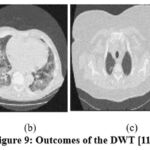Figure 9: Outcomes of the DWT [11].   Click here to view Figure

 

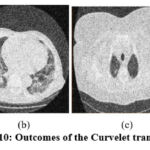Figure 10: Outcomes of the Curvelet transform [12].   Click here to view Figure

 

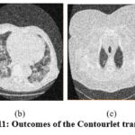Figure 11: Outcomes of the Contourlet transform [13].   Click here to view Figure

 

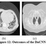Figure 12: Outcomes of the DnCNN [28]   Click here to view Figure

 

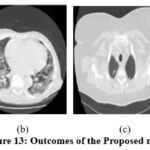Figure 13: Outcomes of the Proposed method.   Click here to view Figure

 

For strong comparison, the noisy CT images are denoised using various approaches, like wiener, median, bilateral, DWT, curvelet transform, contourlet transform, DnCNN, and the proposed method. The performance criteria, including PSNR, SNR, SSIM, ED, and UIQI, are assessed across different noise variances, as presented in Table no. from 1 to 5. The results of the proposed method are highlighted in bold. It is clear from, comparing Tables 1 to 5 that the proposed method outperforms the mentioned standard methods.Table no.1, illustrates comparative analysis of different denoising methods based on PSNR, while Table 2, based on SNR, while Table 3 on SSIM, while Table 4  on ED and Table 5 on UIQI.

Table no.1 shows PSNR results for different denoising approaches applied to four CT images (CT1, CT2, CT3 and CT4) at various gaussian noise levels (𝜎 = 5,10,15,20). The PSNR refers how efficiently the signal is preserved in relation to the level to which its representation has been distorted by noise. The higher PSNR values generally indicates better imaging quality. The proposed method proves to be consistently achieving the highest PSNR values among all mentioned methods. For PSNR, a 0.5% increase in noise results in a considerable decrease of 2-5 points in the PSNR value. SNR measures the ratio between intensity of the desired signal and amount of the noise present in the image. For SNR, increase in noise causes substantial reduction of 1-6 points in SNR value as shown in Table no.2. The method consistently delivers the highest SNR value in comparison with other standard denoising methods.

SSIM is commonly employed to evaluate the imaging quality after compression, denoising, or other processing approaches. It plays a vital role in assessing how well various image denoising algorithms preserve structural information. The SSIM range extends between 0 and 1, with values closer to 1 indicating better denoising performance. For instance, the SSIM values of CT image no. 3 (0.9400) and CT image no. 4 (0.9632) at 𝜎 = 5 are somewhat inferior to those of the proposed method, as shown in Table no.3. CT images with SSIM values greater than 0.80 are considered to be of high quality. It is evident that the proposed method yields superior results compared to existing standard methods in terms of SSIM values.

Table no.4 presents ED values of various denoising methods. A lower ED indicates that the denoising method has well preserved the features of the clean image. The ED values of the Wiener filter for CT image 2 at noise levels 10, 15, and 20 exhibit inconsistent performance, with the ED¹¹ values changing markedly. In CT image 3, the ED⁷ values of the DWT approach are also quite a bit lower compared to the proposed method at noise levels 10, 15, and 20. However, the difference between the proposed method and the outcomes of other standard approaches is quite small. The proposed method consistently outperforms the other denoising techniques in terms of minimizing entropy difference and preserving the original image’s details across various noise intensity levels.

Table no.5 shows a detailed comparison of various denoising methods applied on 4 CT images (CT1, CT2, CT3 and CT4) including proposed method based on UIQI values at different gaussian noise levels (σ = 5,10,15,20). Here, UIQI is used to analyze the quality of denoised-CT images, where higher UIQI value indicates superior image quality. The proposed method performs well at (𝜎 =5) lower noise levels. The proposed technique achieves the highest UIQI values among all standard methods, with DWT and proposed method exhibiting slightly better performance.

The exploratory results of, ⁹ as depicted in Fig. 5 are evaluated, and it is noted that the denoising scheme is performed well but does not effectively preserve structural details at higher noise levels. In the experimental data of ,⁶ as illustrated in Fig. 6, it is observed that the noise suppression is performed effectively, but at higher noise levels, it is unable to preserve the image’s smoothness and edge information in detail. According to the experimental results of,⁷ as demonstrated in Fig. 7, the noise suppression is done effectively. The SSIM of CT3 and CT4 images shows better outcomes at noise variance 5. The experimental findings of,¹⁷ as depicted in Fig. 8, show that noise suppression and other artifacts are reduced successfully, and it is observed that as more noise is added, resulting blurry images.

In the experimental results of,¹¹ as shown in Fig. 9, the noise suppression is performed well, but as the noise increases, it affects image clarity and quality. The experimental outcomes of,¹² as shown in Fig. 10, give superior noise suppression but fail to preserve the image’s structural and fine details at higher noise levels. The ED of the CT2 image at gaussian noise level 10, 20 gives better outcomes. In the experimental results of,¹³ as shown in Fig. 11, the suppression of noise is performed well. If noise variance has increased, the resulting image overall looks blurry. The experimental results of the proposed technique as depicted in Fig. 12, illustrate that the proposed study mitigates noise effectively and also retain edges, other structural, and fine details of an image. The experimental outcomes are tested on different noisy intensities; however, the images are displayed only at noise variance 10.

The proposed algorithm combines NSST with a thresholding function and its noise-based CNN approach. This approach exploits NSST with Bayes thresholding to get denoised NSST coefficients. Here, the NSST domain  provides various  features of an image depicts in different dimensions and different directional subbands. The main benefit of recommended methodology is, applying the method noise-based CNN approach gives better noise reduction and preserves edge’s information. In high textured, noisy CT images, some residuals or the image’s structural and fine details may get damaged during denoising using the NSST domain. To overcome that, the proposed method noise-based approach using CNN gives better performance in order to improve image quality. Performance metrics like PSNR, SNR, SSIM, ED, and UIQI have proven that the proposed method remarkably reduces noise at different noise intensities and also provides better images and fine detail preservation as compared to other denoising techniques. Here, the ED values in the proposed method are near zero. Hence, it has been proven this novel hybrid approach gives improvised outcomes in case of visual clarity, quality, and performance benchmarks.

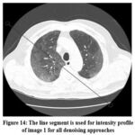Figure 14: The line segment is used for intensity profile of image 1 for all denoising approaches   Click here to view Figure

 

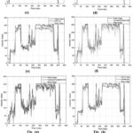Figure 15: Intensity profiles of clean image, noisy image and proposed approach, respectively;   Click here to view Figure

 

(a). Intensity profile of clean image against noisy image and proposed filtered image⁹; (b) Intensity profile of clean image ,noisy image and proposed filtered  image⁶; (c) Intensity profile of clean image ,noisy image and proposed filtered image⁷; (d) Intensity profile of clean image ,noisy image and proposed filtered image¹⁷; (e) Intensity profile of clean image ,noisy image and proposed filtered image¹¹; (f) Intensity profile of clean image ,noisy image and proposed filtered image¹²; (g) Intensity profile of clean image ,noisy image and proposed filtered image¹³; (h) Intensity profile of clean image, noisy image and proposed filtered image²⁸; (i) Intensity profile of clean image, noisy image and proposed filtered image.

Another critical assessment for addressing variations among noisy CT image, clean CT image, and denoised or filtered CT image, is obtaining the pixel’s intensity’s profile. The outcome shows the  clean image, a noisy image (noise variance 10), and a denoised or filtered CT image’s intensity profile as shown in Fig. 14, the lowest difference has been figured out between an original or clean image and proposed denoised image i.e, the ensembled method  provides effective noise suppression as well as preserving edges and fine details.

Conclusion and Future work

The CT images are extensively used in the medical and healthcare domain, as they precisely recognise the abnormality information of the patient. In the proposed work, initially  gaussian noise was added at various levels, ranging in noise variance from 5 to 20. These noise variances are used to estimate the efficacy of various denoising techniques. The proposed study includes NSST and a noise-based CNN method to remove Gaussian noise in CT images. Here, NSST is used as a preprocessing operation to resolve the noisy CT image into various frequency subbands. Bayesian thresholding is applied to denoise noisy NSST coefficients. After denoising NSST coefficients, a postprocessing approach is used to get residuals that were preserved in denoised CT images. The DnCNN was applied to method noise to extract structural information and fine details of CT images. The experimental study employed four CT scan images, i.e., CT2, CT3, and CT4. Standard denoising filters were applied to noisy CT images. All experimental outcomes in proposed method are evaluated against standard methods. So,  the ensembled method gives benchmarked performance in case of PSNR, SNR, SSIM, ED, and UIQI. The proposed study has proven that the experimental results from Table.no. from 1 to 5 and Fig.no. from  5 to 15, shows  better results over the CT imaging from the perspective of visual quality.

For future work, must investigate the integration of advanced deep learning models to further improve denoising effectiveness and enhance computational efficiency. Moreover, broadening the study to encompass a larger and more varied collection of CT images can verify the reliability of the proposed method. Analyzing the use of the technique in various medical imaging modalities such as X-rays or MRI or could expand its applicability. Implementing real-time denoising features would improve clinical practices. Finally, analyzing the effect of denoising on diagnostic precision and patient outcomes would reveal valuable insights and understanding of its practical value.

Acknowledgment

I would like to express my deepest gratitude to my PhD supervisor, Prof. Deepak Garg, for his invaluable guidance, support, and encouragement throughout the course of this research. His insightful feedback and unwavering mentorship have been instrumental in shaping this work. I am equally grateful to my co-supervisor, Dr. Prabhishek Singh, for his constant advice, suggestions, and support, which have been crucial in navigating the complex challenges of this research work. A special thanks to Prof. Manoj Diwakar for sharing his expert knowledge and providing specific insights on CT image denoising, which significantly contributed to the refinement and depth of this research.

Funding Sources

The author(s) received no financial support for the research, authorship, and/or publication of this article.

Conflict of Interest

The authors do not have any conflict of interest

References

1. Albeshan, S., Algamdi, S., Alkhybari, E., Alhailiy, A., Fisal, N., Alsufyan, M., … & Abuhaimed, A. Radiation exposure and cancer risk of pediatric head CT scans: impact of age and scanning parameters. Radiation Physics and Chemistry.2024;216:111459.
   CrossRef
2. Bagherzadeh, S., MirDerikvand, A., & MohammadSharifi, A. Evaluation of radiation dose and radiation-induced cancer risk associated with routine CT scan examinations. Radiation Physics and Chemistry.2024;217:111521.
   CrossRef
3. Zhang, J., Gong, W., Ye, L., Wang, F., Shangguan, Z., & Cheng, Y. A review of deep learning methods for denoising of medical low-dose CT images. Computers in Biology and Medicine. 2024;108112.
   CrossRef
4. Diwakar, M., Singh, P., & Garg, D. Edge-guided filtering-based CT image denoising using fractional order total variation. Biomedical Signal Processing and Control. 2024;92:106072.
   CrossRef
5. Sadia, R. T., Chen, J., & Zhang, J. CT image denoising methods for image quality improvement and radiation dose reduction. Journal of Applied Clinical Medical Physics. 2024;25(2).
   CrossRef
6. Diwakar, M., & Kumar, M. A review on CT image noise and its denoising. Biomedical Signal Processing and Control. 2018;42:73-88.
   CrossRef
7. Zhang, M., & Gunturk, B. K.Multiresolution bilateral filtering for image denoising. IEEE Transactions on image processing. 2008; 17(12):2324-2333.
   CrossRef
8. Li, Z., Yu, L., Trzasko, J. D., Lake, D. S., Blezek, D. J., Fletcher, J. G., … & Manduca, A. Adaptive nonlocal means filtering based on local noise level for CT denoising. Medical physics. 2014;41(1):011908.
   CrossRef
9. Siddiqi, A. A Filter selection for removing noise from CT scan images using digital image processing algorithm. Biomedical Engineering: Applications, Basis and Communications. 2024;36(01):2350038.
   CrossRef
10. Sagheer, S. V. M., & George, S. N. A review on medical image denoising algorithms. Biomedical signal processing and control. 2020;61:102036.
    CrossRef
11. Mallat, S. G.A theory for multiresolution signal decomposition: the wavelet representation. IEEE transactions on pattern analysis and machine intelligence. 1989;11(7):674-693.
    CrossRef
12. Candes, E., Demanet, L., Donoho, D., & Ying, L.Fast discrete curvelet transforms. multiscale modeling & simulation. 2006;5(3): 861-899.
    CrossRef
13. Do, M. N., & Vetterli, M. The contourlet transform: an efficient directional multiresolution image representation. IEEE Transactions on image processing. 2005;14(12):2091-2106.
    CrossRef
14. Kim, K., & Lee, Y. Block-matching and 3D filtering algorithm in X-ray image with photon counting detector using the improved K-edge subtraction method.  Nuclear Engineering and Technology. 2024;56(6):2057-2062.
    CrossRef
15. Li, Z., Yu, L., Trzasko, J. D., Lake, D. S., Blezek, D. J., Fletcher, J. G., … & Manduca, A. Adaptive nonlocal means filtering based on local noise level for CT denoising. Medical physics. 2014;41(1):011908.
    CrossRef
16. Yang, W., Hong, J. Y., Kim, J. Y., Paik, S. H., Lee, S. H., Park, J. S., … & Jung, Y. J.  A novel singular value decomposition-based denoising method in 4-dimensional computed tomography of the brain in stroke patients with statistical evaluation. Sensors. 2020;20(11):3063.
    CrossRef
17. Diwakar, M., & Singh, P. CT image denoising using multivariate model and its method noise thresholding in non-subsampled shearlet domain. Biomedical Signal Processing and Control. 2020;57:101754.
    CrossRef
18. Diwakar, M., Singh, P., Swarup, C., Bajal, E., Jindal, M., Ravi, V., … & Singh, T. Noise suppression and edge preservation for low-dose COVID-19 CT images using NLM and method noise thresholding in shearlet domain. Diagnostics. 2022; 12(11):2766.
    CrossRef
19. Diwakar, M., & Kumar, M. CT image denoising using NLM and correlation‐based wavelet packet thresholding. IET Image Processing. 2018;12(5):708-715.
    CrossRef
20. Chen, W., Shao, Y., Wang, Y., Zhang, Q., Liu, Y., Yao, L., … & Gui, Z. A novel total variation model for low-dose CT image denoising. IEEE Access. 2018;6:78892-78903.
    CrossRef
21. Jifara, W., Jiang, F., Rho, S., Cheng, M., & Liu, S. Medical image denoising using convolutional neural network: a residual learning approach. The Journal of Supercomputing. 2019;75:704-718.
    CrossRef
22. Trung, N. T., Trinh, D. H., Trung, N. L., & Luong, M. Low-dose CT image denoising using deep convolutional neural networks with extended receptive fields. Signal, Image and Video Processing. 2022; 16(7):1963-1971.
    CrossRef
23. Yang, Q., Yan, P., Zhang, Y., Yu, H., Shi, Y., Mou, X., … & Wang, G. Low-dose CT image denoising using a generative adversarial network with Wasserstein distance and perceptual loss. IEEE transactions on medical imaging. 2018;37(6):1348-1357.
    CrossRef
24. Yuan, J., Zhou, F., Guo, Z., Li, X., & Yu, H. HCformer: hybrid CNN-transformer for LDCT image denoising. Journal of Digital Imaging. 2023;36(5):2290-2305.
    CrossRef
25. Han, K., Wang, Y., Chen, H., Chen, X., Guo, J., Liu, Z., … & Tao, D. A survey on vision transformer. IEEE transactions on pattern analysis and machine intelligence. 2022;45(1):87-110.
    CrossRef
26. Abhisheka, B., Biswas, S. K., Purkayastha, B., Das, D., & Escargueil, A. Recent trend in medical imaging modalities and their applications in disease diagnosis: a review. Multimedia Tools and Applications. 2024;83(14): 43035-43070.
    CrossRef
27. Sehgal, R., & Kaushik, V. D. Deep Residual Network and Wavelet Transform-Based Non-Local Means Filter for Denoising Low-Dose Computed Tomography.  International Journal of Image and Graphics. 2024;2550072.
    CrossRef
28. Zhang, K., Zuo, W., Chen, Y., Meng, D., & Zhang, L. Beyond a gaussian denoiser: Residual learning of deep cnn for image denoising. IEEE transactions on image processing. 2017;26(7):3142-3155.
    CrossRef
29. Zhang, J., Niu, Y., Shangguan, Z., Gong, W., & Cheng, Y. A novel denoising method for CT images based on U-net and multi-attention. Computers in Biology and Medicine. 2023;152:106387.
    CrossRef
30. Huang, Z., Chen, Z., Quan, G., Du, Y., Yang, Y., Liu, X., … & Hu, Z. Deep Cascade Residual Networks (DCRNs): Optimizing an Encoder–Decoder Convolutional Neural Network for Low-Dose CT Imaging. IEEE Transactions on Radiation and Plasma Medical Sciences. 2022; 6(8):829-840.
    CrossRef
31. Selig, T., März, T., Storath, M., & Weinmann, A. Low-Dose CT Image Reconstruction by Fine-Tuning a UNet Pretrained for Gaussian Denoising for the Downstream Task of Image Enhancement. arXiv preprint arXiv:2403.03551. 2024.
32. Song, G., Xu, W., & Qin, Y. NeXtResUNet: A neural network for industrial CT image denoising. Journal of Radiation Research and Applied Sciences. 2024;17(1):100822.
    CrossRef
33. Byeon, H., Patel, R. K., Vidhate, D. A., Kiyosov, S., Rahin, S. A., Keshta, I., & Lakshmi, T. V. Non-sample fuzzy based convolutional neural network model for noise artifact in biomedical images. Discover Applied Sciences.2024;6(1):16.
    CrossRef
34. Li, Q., Li, R., Li, S., Wang, T., Cheng, Y., Zhang, S., … & Wang, L. Unpaired low‐dose computed tomography image denoising using a progressive cyclical convolutional neural network. Medical Physics.2024; 51(2):1289-1312.
    CrossRef
35. Çalişkan, A., & Çevik, U. An efficient noisy pixels detection model for CT images using extreme learning machines. Tehnički vjesnik. 2018;25(3):679-686.
    CrossRef
36. Çalışkan, A. Finding complement of inefficient feature clusters obtained by metaheuristic optimization algorithms to detect rock mineral types. Transactions of the Institute of Measurement and Control. 2023;45(10):1815-1828.
    CrossRef
37. Diwakar M, Lamba S, Gupta H. CT image denoising based on thresholding in shearlet domain. Biomed Pharmacol J. 2018;11(2):671-677.
    CrossRef
38. Silverman BW. Wavelets in statistics: beyond the standard assumptions. Philos Trans R Soc Lond A. 1999;357(1760):2459-2473.
    CrossRef
39. Singh, P., Diwakar, M., Gupta, R., Kumar, S., Chakraborty, A., Bajal, E., … & Paul, R.  A method noise-based convolutional neural network technique for CT image Denoising. Electronics, 2022;11(21): 3535.
    CrossRef
40. Abramovich, F., Angelini, C., & De Canditiis, D. Pointwise optimality of Bayesian wavelet estimators. Annals of the Institute of Statistical Mathematics. 2007;59(3):425-434.
    CrossRef
41. Diwakar, M., & Kumar, M. CT image denoising using NLM and correlation‐based wavelet packet thresholding. IET Image Processing. 2018;12(5):708-715.
    CrossRef

(Visited 7 times, 1 visits today)