Anil Kumar Mandle^*, Satya Prakash Sahu and Govind Gupta

Department of Information Technology, National Institute of Technology, Raipur, India

Corresponding Author E-mail: akmandle@gmail.com

DOI : https://dx.doi.org/10.13005/bpj/2409

Abstract

Brain tumor and other nervous systems cancer are one of the leading causes of death for many patients. Magnetic resonance imaging (MRI) is the most important medical imaging modality for diagnosing brain tumors and other disorders in the brain. Manual evaluation of several MRI images by radiologists or experts for diagnosing brain tumors especially at early stages is a challenging task. Hence, this paper proposes an automated framework for the segmentation and classification of brain tumors using K-means clustering and kernel-based support vector machine (K-SVM). The major steps of the proposed framework consist of preprocessing, segmentation, feature extraction with selection, and classification. In the preprocessing step, the regions of interest (ROI) are extracted using skull stripping and a median filter. In the next step, the tumor is segmented using an optimized K-means algorithm. Further, discrete wavelet transform (DWT)-based texture features are used for feature extraction, and significant features are selected by principal component analysis (PCA). Finally, the kernel-based support vector machine (K-SVM) is used for the classification of brain tumor types into benign and malignant, with a dataset using 160 MRI images, consisting of 20 normal and 140 abnormal. Experimental findings demonstrated the efficacy of the proposed framework with 98.75% accuracy, 95.43% precision, and 97.65% recall. The simulation findings emphasize the importance of the proposed system as compared to state-of-the-art techniques in terms of coherence parameters and performance.

Keywords

Brain tumor MRI; DWT; K-means algorithm; KSVM; PCA; Segmentation

Download this article as: 

Copy the following to cite this article: Mandle A. K, Sahu S. P, Gupta G. Brain Tumor Segmentation and Classification in MRI using Clustering and Kernel-Based SVM. Biomed Pharmacol J 2022;15(2).

Copy the following to cite this URL: Mandle A. K, Sahu S. P, Gupta G. Brain Tumor Segmentation and Classification in MRI using Clustering and Kernel-Based SVM. Biomed Pharmacol J 2022;15(2). Available from: https://bit.ly/3NCaSQh

Introduction

Brain tumors might be a dangerous disease for a human. It is a mass or growth of abnormal cells in the brain. In different imaging modalities such as Single-photon Emission Computed Tomography (SPECT), X-ray, Positron Emission Tomography (PET), Computed Tomography (CT), and Magnetic Resonance Imaging (MRI), the MRI has become a very useful medical diagnostic tool for the identification and diagnosis of brain tumors. In addition, MRI provides clear images of various parts of the brain rather than Ultrasound or CT scan and X-ray [1].In recent years, the medical sector has benefited from the implementation of IT and e-health care systems, which allow healthcare experts to deliver quality health care to patients. Kumari et al [2] studied brain MRI classification through feature extraction technique followed by the Support Vector Machine (SVM) classifier to categorize the tumor.

The most popular grading system from Grade-I to Grade-IV of brain tumors distinguishes between benign and malignant tumor types. Benign tumors are classified as grade I and II glioma, while malignant tumors are classified as grade III and IV glioma. Medical imaging modalities are segmented to diagnose compromised tumor tissues [3]. The method of dividing an image into separate regions or blocks that share similar and equivalent properties like color, texture, contrast, brightness, borders, and gray level is known as segmentation. Using MR images or other imaging modalities, from tumor cells like gray matter (GM), brain tumor segmentation identifies tumor tissues such as dead and edema cells GM, white matter (WM), and cerebrospinal fluid (CSF), as well as normal brain tissues. It is apparent that if a tumor-infected patient’s chances of survival are greatly improved when the tumor is diagnosed correctly in the early stages [4]. Therefore, the solution for the best result, the discussing of brain tumors using types of images has been gained importance to the department of radiology.

Although there exist numerous methods for brain tumor classification, they have certain limitations which require being precise while effective with brain tumor segmentation and classification. The first problem in these methods is their binary tumor categorization, which leaves the radiologist with various questions. The reason for this is that a radiologist’s categorization of a tumor as benign or malignant is difficult to determine treatment and prevention options for the patient. For radiologist clarity and comprehension, the classification must be multi-class, which classifies brain tumors into relevant categories. Furthermore, researchers have a significant problem in achieving exact findings because of a lack of data. To address these key limitations, we proposed a kernel-based support vector machine (K-SVM) is applied for the classification of brain tumor types benign and malignant.

The contribution of the proposed methodology is presented below

Preprocessing is the initial step for the median filter to be utilized in which noises present in the images are removed.

Segmentation is performed based on the K-means algorithm. The proposed optimized K-means algorithm overcomes the difficulties present in the traditional approach.

Discrete Wavelet Transform (DWT)-based texture features are used to feature extraction and significant features are selected by the principal component analysis (PCA). This approach is mainly used to reduce complexity and increase accuracy.

The K-SVM-based algorithm is proposed for tumor K-SVM overcomes the difficulties present in the traditional SVM in which accuracy is further improved.

The remaining section of the paper is structured as follows: Section 2 addresses related works, Section 3 described materials and techniques, including proposed method, Section 4 Experimental results and discussion, and Section 5 involve conclusions and future work scope.

Related Works

Segmentation and classification of brain tumors have been carried out in various studies and the most common methods used in these articles are based on classification, clustering algorithms, thresholding, and morphological operations. In [5], for segmentation, Fuzzy c-means has been utilized and for feature extraction, a gray level length matrix is used, and MRI brain images are labeled using the SVM technique with separate kernels. The accuracy results in performances of SVM classification for kernel functions including Linear, Quadratic, and Polynomial. K-means and the Histogram Normalization are segmentation operations. De-noising methods such as the median filter, wiener filter, averaging filter, spatial filter, adaptive filter, and Gaussian filter are used to eliminate noise from the MRI input image during preprocessing. The resultant will then be normalized before being fed into a classifier for classification [6]. After segmentation, the tumor is identified using the k-means algorithm. The magnetic resonance image is carried out using the NB classifier and SVM classifier to achieve more accuracy in estimation and classification. Naive Bayes was used for the classifier, while the best accuracy of the SVM classifier. In comparison to other classifiers, the SVM classifier performs well. Since the tumor area is not exact and reliable, the suggested approach has certain drawbacks on the boundary. SVM is used for classification. Here, the input images must go through a series of steps before being focused on the region of interest (ROI). The SVM is used for classification in this system [7]. It is possible to attain a degree of precision. The best way to segment and identify a tumor in brain MRI images is to use CNN-based image segmentation, pre-processing procedures, and data augmentation. Bias field improvement, intensity, and regular image patches are all part of it. To research deep structures, this device is based on convolution layers 3×3 with kernels [8]. A strategy is planned in [9] a method and classified the MRI brain tumor where the input is 3-D MR images. This method created high-quality results for accuracy, sensitivity, and specificity. For a multiclass brain tumor, a procedure has based on segmentation and feature extraction for images was conferred. A total of 428 MR images were used in this study. The ANN and PCA-ANN methods are used in classification to increase precision [10]. The explained how to solve the image visibility and clearance issue with the fewest possible configuration parameters on the input image [11]. They did this by dividing the medical specialty procedure into two groups of automated procedures. Inset one, they focus on image quality and segmentation of the object of interest, which is a tumor, by forming an edge diagram. In the second package, they performed data analysis by measuring the parameters derived from the diagnosis. The multi-modal hybrid fusion and convolution neural network recognition system was combined in this experiment. The use of the 2D CNN and 3D CNN multimodal extension by having brain lesion with various characteristics in 3D was used in [12] this article. By solving the 2D CNN for various modal details at raw input faults to boost convergence speed, a real normalization layer was added to the convolution and pooling layers to remove the issue of overfitting. Resulting in the improvement of the loss function, so weighted loss function is added in the lesion area to develop the feature learning. The image segmentation method uses the FCM clustering algorithm through a rough set theory. The authors construct the feature values obtained from the FCM segmentation outcome and the image is separated into small areas based on the attribute. Biased values are obtained with value decrease and used for the calculated variation between the region and comparison of the region. Later was realized through similarity variation degree [13]. This final value of equivalence degree is used to evaluate the segmentation of images and combine regions. The method has the limits up to single MRI images of brain and CT, artificially generate images. From the above-mentioned survey, it has been justified that some techniques are designed for segmentation and classification, some are simply for feature extraction, and some are only for classification.

Proposed Methodology

This section presents a detailed work of the proposed framework in which an optimized K-Means algorithm [14] and K-SVM are used for efficient segmentation and classification of the MRI brain tumors. The major step of this work consists of preprocessing, segmentation, feature extraction with selection, and classification. In the preprocessing step, the regions of interest (ROI) are extracted using skull stripping and the noise effects are removed by using the median filter. In the next step, the tumor is segmented using an optimized K-means algorithm. Further, DWT-based texture features are used for feature extraction, and significant features are selected by the Principal Component Analysis (PCA). Finally, the kernel-based support vector machine (K-SVM) is applied for the classification of brain tumor types into benign and malignant. Fig. 1 illustrates the block diagram of the proposed framework in which a sequence of operations is performed such as pre-processing of brain MRI images, image enhancement to increase contrast and brightness, skull stripping operation, segmentation, feature extraction, feature selection, and classification using K-SVM.

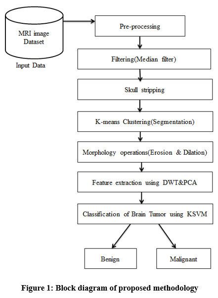Figure 1: Block diagram of proposed methodology. Click here to view figure

Pre-processing Steps

 In this step, the regions of interest (ROI) are extracted using skull stripping and median filter. It improves the accuracy of raw MR images. Furthermore, pre-processing aids in the improvement of certain MR image parameters, such as the signal-to-noise ratio, the removal of irrelevant noise and unwanted bits in the background, the smoothing of the inner part of the area, and the preservation of its edges [15]. To increase the signal-to-noise ratio in our proposed framework.

Median filter

It is a valuable tool for separating out-of-range isolated noise from valid image features like edges and lines to some degree. The median filter replaces a pixel with the median, rather than the average, of all pixels in a neighborhood.

The median filter operates with replacing the value of a pixel with the middle value of the pixels in a little window adjacent to it. For the n×n pixel window, the median filtering operation is represented by the following representation:

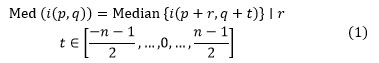
where  i(p,q)-Pixel value at a point (p,q), p,q∈Z.

The threshold is a significant and essential approach to pixel-based segmentation. It is used to transform grayscale pictures into binary images in their most basic form. For segmentation, a threshold value is selected. Pixels with an intensity value less than or equal to the threshold value are changed to black, while those with an intensity value greater than or equal to the threshold value are converted to white. Using Otsu’s technique, the threshold value is determined and converted into a gray image to a binary image.

Image converted get as follow:

where, b₀ and b₁ are for two classes probabilities and divided by a threshold value tv

where, α²₀ and α²₁ are the variances two classes for the calculate the maximum value of α²₀(tv)

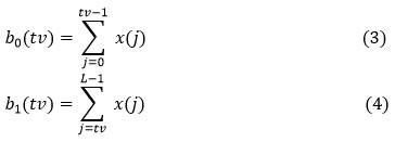
where, b₀ (tv) and b₁(tv) calculated values by the L histogram.

Skull Stripping (SS)

For segmentation for brain tumors, skull stripping is a critical step. It distinguishes between the skull, fat, muscle, and the part of the brain that is not of concern. It eliminates the extra parts of the brain to make the process of segmentation simpler and more efficient. The skull stripping (SS) algorithm [16], which relied on morphological operations, created poor skull stripping and was ineffective when applied to DICOM images. The purpose of skull striping for blob identification and marking system is used in this article. A blog is an area in an image where all the pixels have the same or almost the same properties. All the points in a blob are regarded to be similar in some way and different from their surroundings. The biggest benefit of using blob over the edge and corner detectors is that it produces improved performance and support to provide detailed nearest regions in an image more precisely.

Algorithm: Skull Stripping

Begin 

Step1: Initialize Image I_ij and Q[n] 

Step2: set current label to 1     i.e. curlab=1 

Step3: if (I_ij ==foreground && !=labeled) 

{

Step4:for(i=2, i<n, i++) 

Step5:  labeled= curlab    // labeling of pixel                                    

after first pixel. 

Step6:I_ij = Q_i-1

} 

else (I_ij == background) 

Step7: for all Q[n] 

Implement breadth-first search or depth-first

Search algorithm (to extract neighbor of Q[n]) 

for (k=0,k=n,k++) 

if (Q_k+1=foreground&& Q_k+1 !=labeled) 

Set Q_k+1= curlab

else (Q_k ==background) 

Step8: apply step 3 for all pixels in the Image

Segmentation

Image Segmentation is a procedure of segregating an image into a collection of connected sets of pixels i.e., into regions, linear structures, and 2Dshapes. Image Segmentation is the precise part of the clinical diagnosis. Depending on the image, segmentation can be a very sophisticated process. The segmentation of the infested regions of the MRI brains is attained by the subsequent stages: In the primary step, the pre-processed MR brain image is a binary image converted by the Otsu Thresholding technique [17]. Then in the next stage, the segmentation process will be applied to the binary image. In this study, Enhanced K-means is used for effective segmentation of the brain. The K-means machine learning technique is the best among the most popular partitioning method. In this method, the data is separated into a collectively k finite numeral of clusters and for the allocated each sample it gives the clustered index. In the case of massive data, the K-means clustering is highly deserved than the Hierarchical clustering. The clustering technique K-means is commonly applied for the unsupervised clustering procedure. Understanding the algorithm is easy and a stronghold when making it practice. But it does not provide valid accuracy. So, in this paper, we proposed Enhanced K-means i.e., selecting initial random centers with précising probabilities which increases the speed and also the correctness of the K-means.

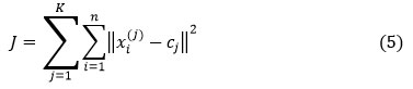
K-means clustering algorithm objective function as follows:

where,

K is the number of clusters, n is the number of cases, x_i is the Case(i), –Centroid cluster j,

and is the distance function.

Algorithm: K-Means Algorithm

Step 1: MSE= large number

Step 2: select initial cluster centroids {c_j}_j^k=1;

Step 3: Do

OldMSE=MSE;

MSE1=0;

for j=1 to k

c_j==0; n_j=0;

endfor

for i=1 to n

For j=1 to n

Step 4:Calculate squared Euclidean

Distance d² (x_i, c_j);

endfor

Step 5:       calculate the closest centroid x_i to c_j

c_j = c_j +x_i; n_j=n_j+1;

Step 6:MSE1=MSE1+d² (x_i, c_j);

endfor

for j=1 to k

Step 7:n_j=max(n_j, 1); c_j=c_j/n_j;

endfor

Step8:MSE=MSE1;

while (MSE<OldMSE)

Pre-processing of the image, extraction of the tumor or ROI, classification of the tumor or that area, and finally, post-processing are all steps in the segmentation of MRI images [18]. K-means algorithm using the improving for the segmentation of low contrast medical images [19], can save time. KSVM can be used to perform region-based classification.

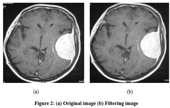Figure 2: (a) Original image (b) Filtering image. Click here to view figure

Morphological Operations

It is used to separate the tumor and the normal region. Morphological operations depend on the pixel’s value, not on the numerical value. It is used to detect the structure of the element [20]. The structure and size of the element will depend on the value zero or one that is represented in the matrix form. The binary or high contract pictures mostly have two types of shading that are white and black. Commonly white represents the foreground image, and black represents the background of the image. Numerically it is denoted as ‘0’ represents black and ‘1 or 255’ used to represent the white region. Fig. 2 and Fig. 3 show Original and filtering images, respectively.

Morphology dilation

Once the de-noised image has been obtained, the morphology dilation is applied on top of the image to extract the tumor region. The dilation works by taking two types of input data. First, it takes the image to be dilated, and secondly structuring element, also known as kernel [21]. The dilation operation adds pixels to the object boundary; the pixels adjoined from the object depend upon the shape and size of the kernel [22]. The final output pixel value will be the maximum pixel value of all the input pixels. We have used dilation since it grows in size and thickens while the holes in the region will become smaller. Once this process is successful the tumor region in the image will be visible (white), the background will be black.  Masking works by assigning some of the pixels in the image to zero (black background) while the rest (kernel) is non-zero [23]. Once the morphology dilation has been successful, we have taken two input data (images) for masking. First, we have taken the image from the output image of the morphological operation. Secondly, the preprocessed MRI image is considered and on successful subtraction from the first and second image, a masked image is obtained. Thus, the masked image further helps in classification and gives accurate accuracy. Fig. 3 shows the Morphology dilation operation.

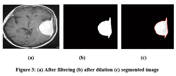Figure 3: (a) After filtering (b) after dilation (c) segmented image. Click here to view figure

Feature Extraction

Feature extraction is the method of gathering an image’s higher-level details, like structure, color, contrast, and texture. Texture analysis is a significant component of both human visual analysis and machine learning techniques. By choosing notable features, it is successfully used to enhance the precision of the diagnostic system.

Discrete Wavelet Transform (DWT)

 It is a linear transformation that converts one data vector into another. The transformed vector’s length is an integer to the second power.DWT divides data into four frequency components [24]. The four levels are Low Low (LL), Low High (LH), High Low (HL), and High High (HH). Many frequency parameters were tested with the appropriate resolution for their respective sizes. Digital filtering algorithms are used to represent the digital signal in time-scale in DWT. The examined signal is allowed to move through filters with varying cutoff frequencies and scales. This signal is compared to the contained basis utilities, which are described as removed and scaled types of any previously set of wavelets. Wavelets get the advantage of providing localized frequency information on a function, such as:

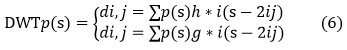
The coefficients of di,j refer to the nearest components, while di,j refers to the element attribute in signal p(s) referring to the wavelet function. There are two High-pass and low-pass filter coefficients (s) and g(s), respectively, while wavelet scale and translation variables are represented by the parameters i and j.

The discrete wavelet transform (DWT) is used in this analysis to remove features from MRI images. The wavelet [25] is an efficient mathematical method for extracting functions. The wavelet transform is particularly useful because it provides knowledge nearby the signal in both the frequency and time domains. Transforming images from the 3-Dfield into the occurrence field. Using DWT, we may fragment an image into levels through their appropriate DWT coefficients. The DWT is performed using flowed decomposition method, with low pass and high pass filters that must fulfill specific criteria. Figure 4 depicts the simple DWT fetidness scheme and its use in MR images. The coefficients of the high-pass as well as low-pass filters are represented by the functions h(n) and g(n), respectively. Therefore, at each scale grade level, there are four levels of imagining (LL, LH, HH, HL).DWT for the decomposition at the next scale, individual the sub-band LL is used for function extraction.

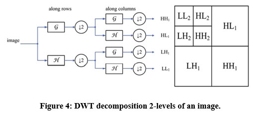Figure 4: DWT decomposition 2-levels of an image. Click here to view figure

Principal Component Analysis (PCA)

PCA is a mathematical procedure for obtaining a reduced number of ages in the knowledge lattice and is useful for obtaining the highest possible values of variance. The entire approach is based on the subject, which generates a large dataset; the database is then analyzed for relations between the set’s independent points. Its basis vectors are the covariance matrix Eigenvectors of the input data. This can be useful when investigating multivariable data processing as new dimensions, referred to as principal components PCs in the dataset. By choosing the PCs with the highest Eigenvalues, a reduced dimension can be obtained [26] fig.5 shows the implementation of PCA.

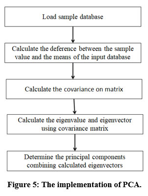Figure 5: The implementation of PCA. Click here to view figure

Mean (M)

A calculated picture is created by multiplying all images’ pixel values with the total number of pixels into the image, and it is expressed as

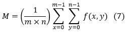
Where n and m are the dimensions of the image a lower value means that the image seems to have a good amount of noise removed.

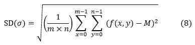
Standard Deviation (SD)

Calculated for the second step central moment there are defines an observed population’s probability distribution and can be used to calculate inhomogeneity by standard deviation. A higher value means a higher level of saturation and high contrast at the image’s edges.

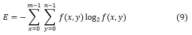
Entropy (E) Entropy is a measure of the random of a textural picture that is calculated and expressed as

Skewness (𝑆𝑘)

Skewness is a measurement of absence there. (X) is the random variable X, and it is defined as

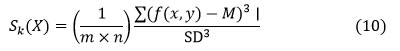
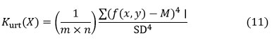
Kurtosis (𝑆𝑘)  

Kurtosis is a parameter that describes the form of random variables in probability distributions. Kurtosis is denoted as Kurt(X) for a random variable X, and it is described as

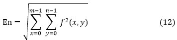
Energy (En)

The energy is a measurable total of the degree of repetitions for pair pixels. Energy is a metric for evaluating how close two images. If Haralick’s GLCM function is used to define energy, it is also known as pointed moment, and it exists expressed as

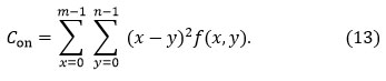
Contrast (𝐶𝑜𝑛). It is defined as the pixel’s intensity and that of its neighbors across a contrasting picture, and it is described as

Inverse Difference Moment (IDM) or Homogeneity

Inverse difference the limited homogeneity of an image is considered with its moment. To decide whether an image is textured or not textured, IDM can have a single value or multiple values.

Directional Moment (DM)

It is described as a measurement of the textural motilities picture utilizing the image’s alignment as a metric in terms of angle.

Correlation (C_orr )

The spatial dependencies between pixels are described by the correlation function, which is defined as

Coarseness (C_ness )

In image textural analysis, coarseness is a roughness measure. The coarser the texture, the higher the coarseness score window size. Coarseness values are lower in fine textures. It is defined as

Classification

Kernel-based Support Vector Machine (KSVM)

 It’s a good tool for data processing and classification, and it’s based on supervised learning. It has a fast-learning speed even when dealing with large amounts of data. It is used to solve grouping problems in two or more groups. It is based largely on the division plane theory. A division plane is a plane that divides a series of data into groups of separate memberships. It is used in the identification and classification of MR brain tumors. The SVM algorithm is used to classify the tumor class shown in the graphic. It consists of two parts: training and testing.

The most frequently used kernel functions are off-linear kernels, quadratic kernels, polynomial kernels, and sigmoid kernels. The expressions for kernel functions are as follows:

Linear kernel

Quadratic kernel

Polynomial kernel

d >0 is the degree of the polynomial.

Sigmoid kernel

RBF kernel

 

Where p_x, p_y represents the inner products of the kernel and ‘z’ is a constant.

Experimental Results And Discussion

This section presents a detailed discussion of the result analysis using both synthetic and actual brain MRI images. Experiments were carried out using MATLAB tool, which was installed in a PC with Windows 10 OS, 4 GB of RAM, and an Intel Core i5 processor. To compare the effectiveness of the proposed framework, four state-of-art methods are used such as K-NN [25], SOM [24], GA [26], and GCNN [28].

Dataset

MRI images of T2-weighted with 256×256 in-plane resolution in the axial plane were obtained from The AANLIB dataset for brain images (http://adni.loni.ucla.edu/), the OASIS dataset for brain images (http://www.oasis-brains.org/), and Harvard Medical School (http://med.harvard.edu/AANLIB/). The T2 model was chosen because, in comparison to the T1 and PET modalities, T2 images had more contrast and clarity. For the experiment, 160 patients’ MRIs were chosen, including 20 normal and 140 abnormal MRIs, as there is one kind of normal brain MRIs and seven types of abnormal brain MRIs in the dataset. Further, 132 cases have been used for training and 28 cases for validation in the 5-fold cross-validation, the outcomes have been shown in Table 4.

K-Fold Cross-validation

Subsequently, the trained classifier on a single dataset can only succeed with high classification precision for that dataset and not for additional datasets. Cross-validation must be incorporated into our system to avoid overfitting. Cross-validation will not improve the classification accuracy in the end; however, it will make the classifier more accurate and generalizable to other datasets.

Segmentation Performance Measures

The suggested unsupervised clustering algorithms for the segmentation of brain tumors are tested using the following performance tests.

Mean squared error(MSE)

The MSE (mean squared error) is a measure of how well everything does. MSE indicates the mechanisms of squaring the distinct principles. The MSE is the average of the number of squares of the defects, which is calculated by subtracting the input image segmented (Fig. 6). MSE may be written as follows:

Where R (a, b) and S (a, b) are respectively input and segmented image.  The total rows and columns from MRI brain image input are m and n. For a better PSNR, the obtained MSE value for the segmented image should be tiny.

PSNR (peak signal to noise ratio)

 The peak signal to noise ratio shows an image’s noise immunity. More PSNR shows that noise disturbance in the MRI brain image is low. The largest pixel value in the input MR brain image is designated as a maxi.

The PSNR is defined by the MSE values. PSNR values in the range of 40 to 100 dB were produced by the algorithm, making it less susceptible to noise. PSNR is commonly expressed as

Structural Similarity Index (SSIM)

Structural Similarity Index (SSIM) stands as a perceptual metric that shows when picture quality is degraded due to data compression, data transmission losses, or another image processing approach. It’s described as

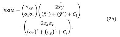
An advanced SSIM value means better luminance, contrast, and structural material preservation.

Dice Coefficient

The dice coefficient, also known as the dice similarity index, is an indicator of when the two images compare, and it is expressed as

Where 𝐴∈ {0, 1} denotes the tumor area as determined by algorithms and 𝐵∈ {0, 1} is the ground truth as determined by experts. The dice coefficient has a minimum and maximum 0, 1 respectively; a higher number indicates that the two images overlap more.

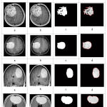Figure 6: (a) Input original image, (b) Threshold for inputted binary conversion, (c) morphological operations, and (d) Segmented image are infected area shows dark white. Click here to view figure

Performance analysis

The features of randomly selected 10 benign samples are shown in Table 1. Fig. 7 shows the result for Graphical representation by the parameters mentioned in Table 1. In Table 2, the features of randomly selected 10 malignant are presented. The graphical representation based on parameters mentioned in Table 2 is shown in Fig 8.

Table 3 shows the definition of the terms for the confusion matrix as TP, TN, FP, and FN.

Table 4 shows 5-fold cross-validation using and their training and validation set to the images.

Table 5 shows the value of MSE, PSNR, and SSIM different techniques.

The graphical findings for the mentioned table 4 are seen in Fig. 9. It shows that, as compared to the approaches described above, the designed approach yields successful results.

The values of precision and recall various methods are shown in Table 6 as TP, FP, TN, and FN.

The graphical findings for the mentioned table 5 are seen in Fig. 10. It was found that the proposed technique outperformed other approaches. The suggested approach is compared to K-NN, SOM, GN, and CNN methods. Fig. 11 shows the graphical performance accuracy comparison of proposed and existing methodologies.

Fig. 12 shows the graphical performance computation time in seconds for comparative analysis.

TP (True Positive): Present tumor that was appropriately identified.

TN (True Negative): Tumor that does not occur and was not detected.

FP (False Positive): recognition of a non-existing tumor.

FN (False Negative): Nearby is an existing tumor that has not been detected. Precision is a metric for determining whether a person has a tumor.

Precision is given by:

The measure of recall is the successful determination of the person not having a tumor.

The specificity is given by:

The measure of accuracy is the successful classification.

The accuracy is given by:

Table 1: feature for randomly selected benign 10 images

Images	means	Standard deviation	Entropy	Energy	Homogen	Contrast	Correlation
Img1	0.00282896	0.0897701	3.62834	0.737835	0.927359	0.215517	0.0950755
Img2	0.0031107	0.0897608	3.17346	0.7621	0.935159	0.208843	0.199005
Img3	0.00348476	0.0897471	3.52392	0.740242	0.926743	0.251669	0.073405
Img4	0.00244646	0.0897814	3.45522	0.747275	0.930409	0.221635	0.134566
Img5	0.0042363	0.0897147	3.03266	0.751967	0.929774	0.264739	0.134791
Img6	0.0020681	0.0897909	3.51816	0.769087	0.936531	0.224972	0.0991065
Img7	0.00341361	0.0897498	3.67835	0.752234	0.930798	0.227197	0.0908294
Img8	0.00348021	0.0897473	3.66808	0.744601	0.929468	0.223026	0.0964256
Img9	0.00234208	0.0897842	3.62596	0.753045	0.932837	0.210512	0.0969614
Img10	0.00229851	0.0897853	3.23654	0.748017	0.932026	0.217186	0.144154

 

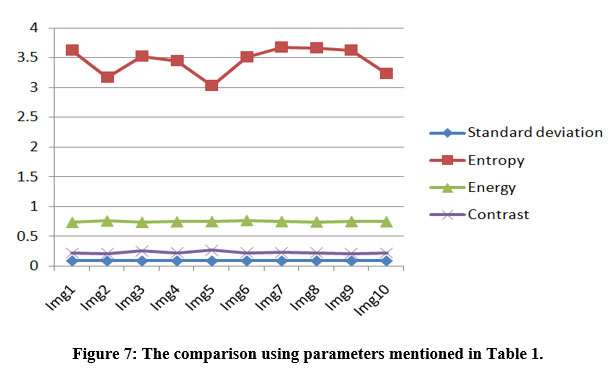Figure 7: The comparison using parameters mentioned in Table 1. Click here to view figure

Table 2: feature for randomly selected malignant 10 images.

images	means	Standard deviation	Entropy	Energy	Homogen	Contrast	Correlation
Img1	0.00346216	0.089748	3.497	0.750879	0.928926	0.244994	0.0948681
Img2	0.00353077	0.0897453	2.75135	0.776902	0.936323	0.299499	0.0910863
Img3	0.00440501	0.0897066	3.18563	0.768842	0.93502	0.25	0.147433
Img4	0.00458293	0.0896977	3.54839	0.731029	0.924625	0.243882	0.107227
Img5	0.00438539	0.0897217	3.37818	0.763092	0.933862	0.265851	0.143025
Img6	0.00440507	0.0897069	3.18565	0.768845	0.93504	0.2576	0.147435
Img7	0.00476278	0.0899883	3.67655	0.755653	0.931929	0.239989	0.0666697
Img8	0.00447512	0.0897066	3.18563	0.768845	0.93505	0.2523	0.147453
Img9	0.00456293	0.0895977	3.54939	0.731027	0.924623	0.243885	0.107223
Img10	0.00469539	0.0898217	3.37518	0.763099	0.933868	0.265854	0.143027

 

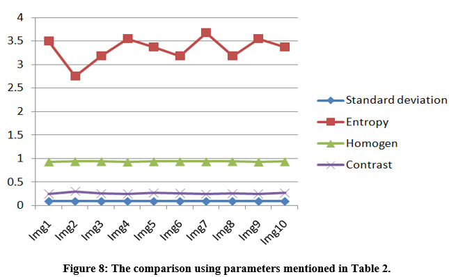Figure 8: The comparison using parameters mentioned in Table 2. Click here to view figure

Table 3: TP, TN, FP and FN used for Confusion Matrix terms.

Result	Negative	Positive	Total
Negative	TN	FN	TN+FN
Positive	FP	TP	FP+TP
Total	FP+TN	TP+FN	FP+TN+ TP+FN

Table 4: Training and validation images preparing (5-fold cross-validation).

Total no. of images	Training (128)		Validation (32)
	Normal	Abnormal	Normal	Abnormal
160	16	112	4	28

Table 5: Parameters for segmented tissue performance.

Methods	MSE	PSNR	SSIM	Dice score
K-NN[25]	0.234	0.75	0.8761		0.81
SOM[24]	0.21	0.76	0.9101		0.83
GA[26]	0.026	0.78	0.9706		0.85
GCNN[28]	0.0324	0.89	0.9863		0.89
Proposed method	0.0012	0.98	0.9901		0.94

 

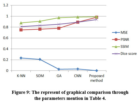Figure 9: The represent of graphical comparison through the parameters mention in Table 4. Click here to view figure

Table 6: compassion of accuracies in different clarifiers methodology.

Methods	TP	FP	TN	FN	Precision	Recall	Accuracy
K-NN[25]	0.8923	1.1441	0.851	1.3843	0.7974	0.9472	0.8503
SOM[24]	0.9213	0.8122	0.893	1.2123	0.8054	0.9654	0.9154
GA[26]	0.9342	0.7642	0.924	0.8765	0.8443	0.9586	0.9767
GCNN[28]	0.9423	0.1123	0.942	0.1654	0.9324	0.9652	0.9589
Proposed method	0.9854	0.0121	0.985	0.0176	0.9543	0.9765	0.9875

 

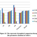Figure 10: The represent of graphical comparison through the parameters mention in Table 6. Click here to view figure

 

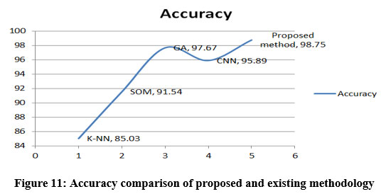Figure 11: Accuracy comparison of proposed and existing methodology. Click here to view figure

 

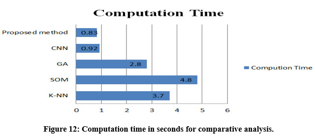Figure 12: Computation time in seconds for comparative analysis. Click here to view figure

Discussion

The proposed approach is quite likely to create more effective results than the existing mentioned techniques. The following are some of the outcomes of the experiment:

The suggested method extracts more information to characterize the ROI more properly.

The recommended technique produces significantly better results than the other techniques mentioned.

The image quality has not been degraded by the proposed technique.

Future development in the approach could involve the following:

The proposed work may be tested and extended for other public databases such as PASCAL, Berkeley, or BRATS.

To develop the performance of the proposed method, some hybrid approaches with different classifiers can be tested in the future.

Conclusion and Future Work

This paper has proposed an efficient automated brain tumor segmentation and classification framework using K-means clustering and kernel-based support vector machine (K-SVM). The major steps of this work consist of preprocessing, segmentation, feature extraction including selection, and classification for brain tumors. The regions of interest (ROI) are extracted using skull stripping and median filter. Discrete Wavelet Transform (DWT)-based texture features are used to feature extraction and significant features are selected by the principal component analysis (PCA). Kernel-based support vector machine (K-SVM) is applied for the classification of brain tumor types into benign and malignant. Result analysis confirms the efficiency of the proposed framework for classifying the benign or malignant tissues using brain MRI images, with 98.75% accuracy, 95.43% precision, and 97.65% recall. The simulation findings emphasize the importance of the proposed approach is compared to state-of-the-art techniques, in terms of accuracy, precision, and recall. In future work, we plan to evaluate the classifier’s selective scheme by integrating several classifiers and feature selection processes.

Acknowledgement

The authors would like to thank Dr. Yashwant Kurmi, Madhyanchal Professional University Bhopal M.P. for the necessary support to do this study.

Conflict of Interest

The authors complete not have any conflict of interest.

Funding Source

This learning received no external funding.

References

1. Guo, Lei, et al. “Tumor detection in MR images using one-class immune feature weighted SVMs.” IEEE Transactions on Magnetics10 (2011): 3849-3852.
   CrossRef
2. Kumari, Rosy. “SVM classification an approach on detecting abnormality in brain MRI images.” International Journal of Engineering Research and Applications4 (2013): 1686-1690.
3. Gordillo, Nelly, Eduard Montseny, and Pilar Sobrevilla. “State of the art survey on MRI brain tumor segmentation.” Magnetic resonance imaging8 (2013): 1426-1438.
   CrossRef
4. Demirhan, Ayşe, Mustafa Törü, and İnanGüler. “Segmentation of tumor and edema along with healthy tissues of brain using wavelets and neural networks.” IEEE journal of biomedical and health informatics4 (2014): 1451-1458.
   CrossRef
5. Hamad, Yousif Ahmed, Konstantin Vasilievich Simonov, and Mohammad B. Naeem. “Detection of brain tumor in MRI images, using a combination of fuzzy C-means and thresholding.” International Journal of Advanced Pervasive and Ubiquitous Computing (IJAPUC)1 (2019): 45-60.
   CrossRef
6. Singh, Garima, and M. A. Ansari. “Efficient detection of brain tumor from MRIs using K-means segmentation and normalized histogram.” 2016 1st India International Conference on Information Processing (IICIP). IEEE, 2016.
   CrossRef
7. Shree, N. Varuna, and T. N. R. Kumar. “Identification and classification of brain tumor MRI images with feature extraction using DWT and probabilistic neural network.” Brain informatics1 (2018): 23-30.
   CrossRef
8. Pereira, Sérgio, et al. “Brain tumor segmentation using convolutional neural networks in MRI images.” IEEE transactions on medical imaging5 (2016): 1240-1251.
   CrossRef
9. Deepa, S. N., And B. Arunadevi. “Extreme Learning Machine For Classification Of Brain Tumor In 3d Mr Images/Elm Za Klasifikaciju Tumora Mozga Kod 3d Mr Snimaka.” Informatologia2 (2013): 111.
10. Sachdeva, Jainy, et al. “Segmentation, feature extraction, and multiclass brain tumor classification.” Journal of digital imaging6 (2013): 1141-1150.
    CrossRef
11. Zotin, Alexander, et al. “Edge detection in MRI brain tumor images based on fuzzy C-means clustering.” Procedia Computer Science126 (2018): 1261-1270.
    CrossRef
12. Li, Ming, et al. “Brain tumor detection based on multimodal information fusion and convolutional neural network.” IEEE Access7 (2019): 180134-180146.
    CrossRef
13. Huang, Hong, et al. “Brain image segmentation based on FCM clustering algorithm and rough set.” IEEE Access7 (2019): 12386-12396.
    CrossRef
14. Poteraş CM, Mihăescu MC, Mocanu M. An optimized version of the K-Means clustering algorithm. In 2014 Federated Conference on Computer Science and Information Systems 2014 Sep 7 (pp. 695-699). IEEE.
    CrossRef
15. Alfonse, Marco, and Abdel-Badeeh M. Salem. “An automatic classification of brain tumors through MRI using support vector machine.”  Comp. Sci. J40.3 (2016).
16. Yogalakshmi, G., and B. Sheela Rani. “A Review On The Techniques Of Brain Tumor: Segmentation, Feature Extraction And Classification.” 2020 11th International Conference on Computing, Communication and Networking Technologies (ICCCNT). IEEE, 2020.
    CrossRef
17. Sharif, Muhammad, et al. “An integrated design of particle swarm optimization (PSO) with fusion of features for detection of brain tumor.” Pattern Recognition Letters129 (2020): 150-157.
    CrossRef
18. Moeskops, Pim, et al. “Adversarial training and dilated convolutions for brain MRI segmentation.” Deep learning in medical image analysis and multimodal learning for clinical decision support. Springer, Cham, 2017. 56-64.
    CrossRef
19. Sahu, Satya Prakash, et al. “Segmentation of Lungs in Thoracic CTs Using K-means Clustering and Morphological Operations.” Advances in Biomedical Engineering and Technology. Springer, Singapore, 2021. 331-343.
    CrossRef
20. Menze, Bjoern H., et al. “The multimodal brain tumor image segmentation benchmark (BRATS).” IEEE transactions on medical imaging10 (2014): 1993-2024.
21. Prastawa, Marcel, et al. “A brain tumor segmentation framework based on outlier detection.” Medical image analysis3 (2004): 275-283.
    CrossRef
22. Singh, Amritpal. “Detection of brain tumor in MRI images, using combination of fuzzy c-means and SVM.” 2015 2nd International Conference on Signal Processing and Integrated Networks (SPIN). IEEE, 2015.
23. Hiremath, P. S., S. Shivashankar, and Jagadeesh Pujari. “Wavelet based features for color texture classification with application to CBIR.” International Journal of Computer Science and Network Security9A (2006): 124-133.
24. Logeswari, T., and M. Karnan. “An improved implementation of brain tumor detection using segmentation based on hierarchical self organizing map.” International Journal of Computer Theory and Engineering4 (2010): 591.
    CrossRef
25. Vrooman, Henri A., et al. “Multi-spectral brain tissue segmentation using automatically trained k-Nearest-Neighbor classification.” Neuroimage1 (2007): 71-81.
    CrossRef
26. Kharrat, Ahmed, et al. “A hybrid approach for automatic classification of brain MRI using genetic algorithm and support vector machine.” Leonardo journal of sciences1 (2010): 71-82.
27. Ouseph, N. C., and K. Shruti. “A reliable method for brain tumor detection using cnn technique.” National Conference on Emerging Research Trends in Electrical, Electronics & Instrumentation (ERTEEI’17). 2017.
28. Mittal, Mamta, et al. “Deep learning based enhanced tumor segmentation approach for MR brain images.” Applied Soft Computing78 (2019): 346-354.
    CrossRef