Careena ¹, M. Mary Synthuja Jain Preetha ² and P. Arun³

¹Department of Electronics and Communication Engineering, Amal Jyothi College of Engineering, Kanjirapally - 686518.

²Department of Electronics and Communication Engineering, Noorul Islam University, Nagercoil- 629180

³Department of Electronics and Communication Engineering, St. Joseph’s College of Engineering and Technology, Palai-686 579.

Corresponding Author E-mail: careenaarun@gmail.com

DOI : https://dx.doi.org/10.13005/bpj/1918

Abstract

Automated identification of valve ailments from heart sound is a popular method an is a skilled task in cardiology. However, the automated methods, mainly depend upon the features extracted from the heart signal. The analysis of Phonocardiogram (PCG) signals, supply significant data about the heart functioning. In this paper, the significance of frequency domain features of Phonocardiogram (PCG) records for murmur detection is inspected. Frequency domain features like Dominant Frequency (DF), Spectral Centroid (SC), Spectral Flux (SF), Spectral Role-off (SR) and Median Frequency (MF), may be used in Artificial Intelligence (AI) to replicate the physical aspects of signals. The first three features are detected directly from the preprocessed heart signal, and the last two features are calculated from the Power Spectral Density (PSD) by means of an analytical method. It has been noticed that, among the features, MF and SR are superior to detect the presence of murmur than others. Besides, they are statistically more significant than all other features. The MF and SR can identify the murmur with an accuracy of 87.35% (dataset1), 76.67% (dataset2) and 80.59% (dataset1), 78.33% (dataset2), respectively without using any classifiers.

Keywords

Dominant Frequency; Frequency Domain Features; Heart Abnormality; Murmur; Median Frequency; PCG Signal; Spectral Centroid; Spectral Flux; Spectral Roll-Off

Download this article as: 

Copy the following to cite this article: Careena P, Preetha M. M. S. J, Arun P. Significance of Frequency Domain Features of PCG Records for Murmur Detection - An Investigation. Biomed Pharmacol J 2020;13(2).

Copy the following to cite this URL: Careena P, Preetha M. M. S. J, Arun P. Significance of Frequency Domain Features of PCG Records for Murmur Detection - An Investigation. Biomed Pharmacol J 2020;13(2). Available from: https://bit.ly/2MGBD9n

Introduction

The feature extraction is one of the important steps in any artificial intelligence framework. Signal processing techniques employed for separating the features assume a vital role in schemes implied for automated study like fault identification of mechanical systems from the vibration data, problem finding of the electrical systems by considering various signals and detection of diseases by examining various biological signals, etc., From the statistically significant and computationally competent features, extracted through proper signal processing procedures, flaws can be accurately traced, detected, and even their type can be recognized. The features will be of time domain, frequency domain, or Time-Frequency (TF) domain.

Coronary artery disease (CAD) is one of the main sources of death and ill health worldwide.  As per the report of World Health Organization (WHO), an expected 17.9 million individuals passed on from Cardio Vascular Disease (CVD) in 2016, representing 31% of all worldwide deaths. Of these deaths, 85% are because of heart attack and stroke [1]. The investigations based on the features acquired from the preprocessed PCG signal may be utilized to spot the presence of CVD from it [2].

In view of the similarity to the human audition, the frequency domain features have comparatively of a higher impact than that of time domain and TF domain. But, the statistical significance of the frequency domain features depends on how powerfully the attributes of the spectrum is converted into numerical indices. It is a general understanding that, if the heart turns unusual, additional frequency components will be overlapped with the inherent frequency components of the normal heart signal. In this paper, the importance of frequency domain features for distinguishing normal heart sound and murmur is proposed.

A few methods that incorporate frequency domain features to identify and solve the cardiac problems are introduced in the literature [3-21]. Surrel et al. [3] introduced an embedded wearable system for detecting the cardiac failure by observing obtrusive sleep apnea by considering the live Electro Cardio Gram (ECG) record. They were computed the frequency spectrum of the RR-interval and RS-amplitude of the unfiltered ECG data. Further, they have also evaluated the relative energy in a specific frequency band among them (accuracy 88.2% for Support Vector Machine (SVM) classifier). Wang et al. [4] suggested a procedure to identify congestive heart failure patients. They have utilized the features like normalized low and high-frequency power, and their ratio obtained from the frequency spectrum of the preprocessed PCG signal by means of autoregressive (AR) process. The features like, very low and high frequency, power very-low-frequency, power low-frequency, and power high-frequency components computed from the spectrum of the ECG signal has been employed in the method put forth by Isler et al. [5]. Al-Zaiti et al. [6] estimated the efficacy of ECG signal in envisaging cause-specific death in patients having very high risk of sudden cardiac arrest. The features were, normalized low- and high-frequency power of the spectrum of the ECG signal. By analyzing PCG, Hamidi et al. [7] investigated that the power spectrum of the curve fitted signal and the fractal dimension of two equally divided PCG signal can be used for the detection of heart abnormality. The features were input into KNN classifier. Average accuracy of 90 % was reported. Bozkurt et al. [8] suggested a scheme to identify the heart abnormality by the feature, Mel-frequency cepstral coefficient (MFCC). The feature extraction has been done after preprocessing and segmentation of the Phonocardiogram (PCG) signal. The features were applied into the Convolutional Neural Network (CNN) for classification. The MFCC based system reported an overall accuracy of 67.17%. A smartphone based electronic stethoscope that can even record, process, and detect heart sounds has been devised by Thiyagaraja et al. [9]. The S1 and S2 heart sound were detected (after preprocessing) with peak detection and a classification model utilizing the Mel-Frequency Cepstral Coefficient and Hidden Markov Model were introduced to detect normal/murmur (accuracy of 80.76% and 92.68 %, respectively). Chen et al. [10] Offered a scheme to detect coronary disease by using bispectrum of the preprocessed ECG signal. They were also stated that, in the bispectrum, the normal heart signal has a lower frequency component than the abnormal heart signal. Kang et al. [11] developed a system for automatic identification of Still’s murmur in children by using spectral width and peak frequency of S1 and S2 heart sound (sensitivity of 84-94% and a specificity of 91-99%). These features were given as input to SVM classifier. In the method suggested by Varghese and Ramachandran [12], the PCG signal decomposition by Empirical Wavelet Transform (EWT) has been done initially. The heart sound/murmur detection was done by Shannon entropy and instantaneous phase after discriminating them using mode boundary frequency and maximum absolute amplitude (accuracy of 91.92%). To predict the Cardiovascular disorder in Type 2 Diabetes patients, Cha et al. [13], utilized the spectral features like total power, low-frequency power and high-frequency power of the preprocessed ECG signal. Sharma et al. [14], projected a system to identify heart failure using heart rate variability analysis of ECG signal. From the eigenvalue decomposed components of ECG signals, the lowest and highest frequency components were extracted. After that, the mean frequency of the decomposed components was estimated via Fourier-Bessel series expansion. The feature was served to least-squares support vector machine (LS-SVM) classifier and produced an accuracy of 93.33%, the sensitivity of 91.41%, and specificity of 94.90%. Fahad et al. [15], implemented a technique for diagnosing cardiac valve disorder. The frequency domain features such as systole and diastole frequency components were estimated from the preprocessed ECG signal spectrum and were given as input into an adaptive neuro-fuzzy inference system (ANFIS) system (Accuracy 98.70%).

The AR models offer comparatively poor performance for short data records. As most of the biological records are of a short span, the schemes using AR models may deteriorate the system performance.  In curve fitting, the number of component peaks bears a significant role to ensure the performance of the system [16]. Hence reasonable prior knowledge on the number of components is required. Although the choice of the right peak half-widths is a vital factor in confirming the success of quantitative curve fitting. The principle challenges in ordinary MFCC are its computational complexity, the robustness of the features in designing the appropriate filter bank, and the poor performance in the existence of noise. One of the restrictions found in EMD is; it has a low-frequency resolution, which indicates that the EMD can reflect only distant spectral components changing by more than an octave. EMD could not do well for smaller amplitudes of the second harmonics and cannot differentiate closely spread out frequencies. It is being understood that the bi-spectrum is a bi-dimensional complex function, represented by a complex matrix. Consequently, it entails an enormous computation. In some cases, the time-efficient computation of bi-spectrum is unpractical for a huge amount of data, and the two-dimensional spectral representation of bi-spectrum may be challenging to interpret.

The approaches mentioned in the literature cannot account directly for the qualitative behavior of the bio signal spectra. The features utilized for classifying various abnormalities should be able to adequately interpret the qualitative attributes of the spectrum, clearly from the visual examination to a reduced set of numerical indices. Besides, before applying the features for various application, the separability and the inter-class variability among them should be checked.

In this paper, the significance of frequency domain features for differentiating normal heart sound and murmur is inspected. The features used are Dominant Frequency (DF), Spectral Centroid (SC), Spectral Flux (SF), Spectral Role-off (SR) and Median Frequency (MF). The highlights of this work are, (a) The frequency domain features proposed are reasonably simple (b) The statistical significance of the features are quantitatively examined using Kolmogorov–Smirnov test (c) The separability among the features are considered via histogram. (d) These features can directly reproduce the Qualitative attributes of the PCG signal spectra. Rest of the paper is structured as follows. The details of the PCG signal database utilized in the analysis and the mathematical representation of frequency domain features and are provided in section 2. The statistical significance of frequency domain features to detect the murmur from the PCG signal is studied in section 3.

Methodology

Heart Murmurs are basically swishing or whooshing sounds during the cardiac cycle caused by turbulent blood in or near the heart and can be present by birth or develop later in life. A heart murmur isn’t a disease however may be an indication of some underlying cardiac issues. Mainly murmurs are classified as innocent and abnormal. An individual having innocent murmur has a normal heart and it is common in infants and children. It happens when blood flows more quickly than typical through the heart during physical action or exercise, pregnancy, fever, hypothyroidism and so on. But the abnormal heart murmur is more dangerous and is mostly due to the inborn heart defects. The defects are holes in the heart or cardiac shunts and valvular abnormalities. Another sources are valve calcification and prolapse, septal defects, rheumatic fever and endocarditis. A few factors that builds the possibility of evolving murmur are family history of a heart defect, certain ailments like hypertension, hyperthyroidism, pulmonary hypertension etc., disease and certain medications during pregnancy period. It is also noted form the literatures that Men have a higher incidence of heart failure than women, but the overall prevalence rate is similar in both genders, since women survive longer after the onset of heart failure [17].

In this paper, the analysis of the PCG records is observed on the two public heart sound data bases, namely, pascal heart sounds challenge database (Pascal HSDB) [18] and physionet heart sound database (Physionet HSDB) [19]. For the analysis, a total of 400 records were selected. In this, 340 records (equally divided murmur and normal signal) from Physionet HSDB (dataset 1) and 60 records from Pascal HSDB (dataset 2). Out of the 60 records of dataset 2, 30 records are normal, and 30 records are murmur. The length of all these .wav format records (sampling frequency 4 KHz) of Pascal HSDB differs from 1 second to 30 seconds and that of Physionet HSDB (sampling frequency 2 KHz) varies from 5 to 120 seconds.

The signals are selected in such a way that each record have sample length more than 8 seconds and are upsampled by a factor 2, ie, the sampling frequency ‘f_s’ of the first dataset is 8 KHz and that of the second dataset is 4 KHz. The frequency components less than 10 Hz are eliminated by a high pass filter (cut off frequency 10 Hz).

Before the computation of the spectral features of the PCG signal must be transformed into the frequency domain. The diagram of the processes involved in the calculation of frequency domain features and feature evaluation is supplied in fig.1.

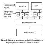Figure 1: Diagram of the processes involved in the calculation of frequency domain features  Click here to View Figure

Prior to the estimation of the frequency domain features, the PCG signal needs to be preprocessed. The schematic of the steps involved in the preprocessing stage is presented in fig.2.

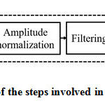Figure 2: The schematic of the steps involved in the preprocessing stage. Click here to View Figure

The role of each block shown in fig.2 is as follows. To attain a sufficient sampling rate, the PCG records are upsampled by a factor 2. The undesirable characteristics of the heart signal have been avoided via offset elimination. To keep all the data samples to a stable level, they are normalized between -1 and +1. Normally, the heart signal frequency components are existing between 10Hz to 2500Hz. The high pass filter removes the frequency components below 10 Hz. To uphold sufficient spectral resolution, using zero padding, the number of samples in the PCG records are raised to at least two times of the sampling frequency ‘fs.’ Zero padding may induce ripples in the spectrum during the computation of FFT. To overcome this, the PCG records are windowed with Hanning window before FFT computation.

The mathematical formulations involved in the computation of frequency domain features are given below. The upsampled offset eliminated heart signal is given as

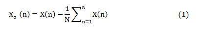
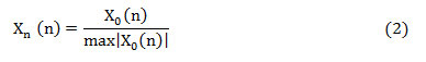
where ‘X(n)’ is the upsampled heart signal (sampling rate ‘1/fs’) and consists ‘N’ samples, 1≤n≤N. This samples are standardized to a range between -1 and +1 as given in (2).

The normalized signal after windowing can be given as,

The mathematical representation of the Hanning window is given by,

 

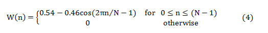
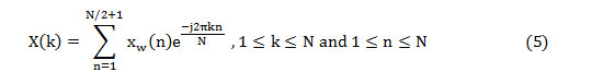
The first half of the spectrum (range from 0 to the Nyquist frequency ‘fs/2’ is sufficient to perceive the frequency components since the second half is only a replication of the first half. The half-length spectrum of the windowed signal ‘Xw(n)’ is calculated as [20-21],

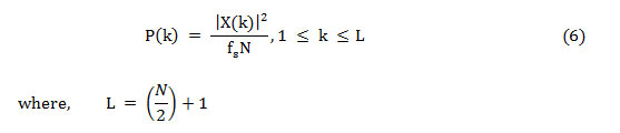
The frequency domain features, namely SF, SC, and DF, can be assessed from the half-length spectrum. But the other two features are computed from the PSD estimation (P(k)) and can be obtained as,

 

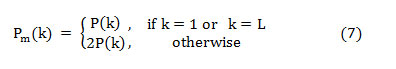
As Nyquist frequency and DC do not occur twice, to save the absolute power, the power spectrum is altered and named as the modified power spectrum,

The PSD approximation is given in dB/Hz,

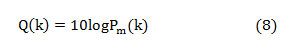
The median frequency can be estimated from the cumulative PSD estimate as extracting this feature from the normal PSD is not promising. The cumulative PSD estimation [20-21],

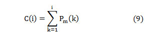
The entire power in the spectrum gets equally distributed at the median frequency [20],

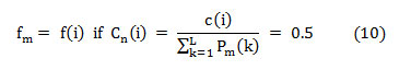
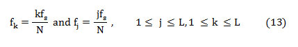
Where ‘Cn(i)’ is the normalized cumulative PSD estimation. The frequency vector analogous to the half-length spectrum,

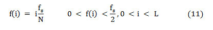
That means, on median frequency ‘f (i),’

In this article, the median frequency is estimated based on an understanding that the magnitude of the normalized cumulative PSD crosses 0.5 strictly at the median frequency. This also reveals the frequency band at which the energy of the spectra is focused.

The feature Spectral roll off [22] is the frequency below which 95% of energy is concentrated. Systematically, it is the frequency at which normalized cumulative PSD exceeds 0.95.

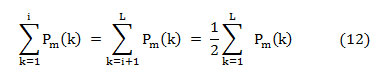
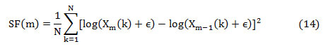
Spectral flux (SF) is the average deviation of the spectral magnitude among two neighboring signal divisions. For the estimation of SF, the signal is separated to ‘M’ segments each comprising ‘N’ samples. The spectral flux (SF) between two adjacent signal segments ‘X_m’ and ‘X_m-1’ is given by,

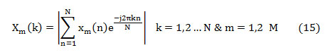
where ‘Xm(k)’ is the absolute spectrum of the m^th segment represented as,

The feature, spectral centroid (fc) is the summation of frequency components weighted by the comparative spectral magnitude of each frequency component to the total spectral magnitude. It is computed as [22],

Where ‘ϵ’ is a small constant used to eliminate computational uncertainty. The overall spectral flux of the signal is estimated by averaging the SF among neighboring segments,

As the dominant frequency is defined as the frequency component that carries more energy concerning all other frequencies in the spectra and is shown as,

The statistical significance of the features is tested for their ability to differentiate normal and murmur using Kolmogorov–Smirnov test. This is a non-parametric hypothesis test employed to quantitatively analyze how far the features differ from each other, especially in binary classification problem. The histogram is also used to evaluate the separability offered by the features. The feature extraction and their statistical interpretation are done by Matlab®.

Results and Discussions

As stated earlier, the features like spectral flux, spectral centroid, and dominant frequency are calculated directly from the preprocessed PCG records. Whereas, the spectral roll off and the median frequency are computed using an analytical technique using the PSD estimation of the heart signal. For visual inspection, the normalized cumulative power spectrum and half-length spectrum of PCG signal of normal and murmur of both datasets are shown in fig. 3 – fig. 6.  The cumulative power spectrum and the half-length power spectrum of normal and murmur is different in their pattern.

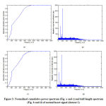Figure 3: Normalized cumulative power spectrum Click here to View Figure

The power spectrums of normal heart signal shown in fig.3 (a) and 3(c) have some similarity in their pattern, but their slopes are changing at different frequencies. By the visual inspection of the power spectrum of normal, it is inferred that the unexpected deviation in the slope happens at low frequencies. The mid-frequency components do not give more to the total power in the normal records. At frequencies almost above 1000 Hz, the slope is zero. From the half-length spectrum of normal heart signal (fig.3 (b) and 3(d)), the magnitude of spectral coefficients is superior at frequencies around 200 Hz and are tightly packed. The spectral magnitude is almost the same between the frequencies 200 Hz to 1000Hz, and above 1000Hz the magnitude gets reduced slowly. The power spectrums of murmur displayed in fig.4 (a) and 4(c) are similar in their pattern, but their shape of slopes are almost same, but it has some alteration at a frequency almost at 200Hz. Above this frequency, slope is stable. From the fig.4(b and d), it has observed that, the frequency of the signal is between 0-2000 Hz. Of this, the spectral magnitude is existing up to 700Hz for the spectrum of the signal shown in fig.4(b) and above 700Hz, the spectral amplitude is very less. Similarly, for fig.4(d), the spectral magnitude is existing almost up to 850 Hz and above that the spectral amplitude is very less. The magnitude spectrum is shown in the fig.4 (b) and 4(d) has an exponential variation in its pattern. The spectral amplitude is higher at low frequency, and are exponentially reduced to a low value as the frequency increases. Moreover, the frequency components are tightly packed than the normal heart signal.

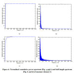Figure 4: Normalized cumulative power spectrum Click here to View Figure

The power spectrums of normal heart signal of dataset 2 shown in fig.5 (a) and 5(c) exhibits similar pattern, however whose slopes have a slight change at low frequencies. By visual examination of the power spectrum of normal, it has inferred that, the slope is zero at frequencies above 500Hz. In the half-length spectrum of normal heart signal (fig.5 (b) and 5(d)), the magnitude of spectral coefficients is dominating at low frequency region. At high frequencies the spectral amplitude is less and it is loosely packed.

Figure 5: Normalized cumulative power spectrum Click here to View Figure

The power spectrums of murmur displayed in fig.6 (a) and 6(c) also has a similar pattern, but a dissimilarity in the slope pattern is noticed. That means, the slope becomes zero at frequencies almost above 700 Hz. In the power spectrums of murmur, only high-frequency components contribute more to the total power. The magnitude spectrum shown in fig.6 (b) and 6(d), the frequency components are tightly packed than that of the normal heart signal. Moreover, the spectral magnitude is also higher than that of the normal heart signal.

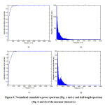Figure 6: Normalized cumulative power spectrum Click here to View Figure

It is understood that from the visual inspection of the power spectrum of the signal of two datasets, the slope of the power spectrum of the normal heart signal reduces at low frequencies when compared with that of the murmur. That means, in case of the cumulative power spectrum of the normal heart signal, the slope is reducing to 0 from its maximum at low frequency ranges than that of the cumulative power spectrum of murmur. Besides, can also be possible to differentiate normal and murmur by visually reviewing the power spectrum, especially by noticing the variation in the slope pattern. It has also noted that the magnitude spectrum of normal heart signal is different than that of the murmur. Its spectral amplitude is exponentially varying. These results reveal that both the slope based features and the spectral amplitude can be useful to differentiate normal heart sound from Murmur.

The range and numerical values of all the features extracted from the heart sound analogous to normal and murmur are presented in Table 1.

From Table 1 it is noticed that, for dataset1, the range of normal heart sound are 23 to 877, 11 to 88, 61.17 to 467.35,10 to 211 and 4.82 to 353.26 for the spectral roll-off, median frequency, spectral centroid, dominant frequency, and spectral flux, respectively. The range of the murmur of the above said dataset ranging from 43 to 170,18 to 50,61.02 to 322.05,11 to 51 and 0.56 to 226.76. The range of features like spectral roll-off, median frequency, spectral centroid, dominant frequency and spectral flux of the normal sound of dataset 2 is 112 to 323,46 to 85,188.70 to 322.46,21 to 120 and 5.87 to 471.44, respectively. For the same dataset the above said features of the murmur ranging from 120 to 597, 52 to 216,192.77 to 468.54,27 to 174 and 8.76 to 273.40.

Table 1: Numerical values and range of features of normal heart sound and murmur

Sl. No	Features	Type	Dataset 1		Dataset 2
			Range	Numerical value	Range	Numerical value
1	spectral roll off	Normal	23 to 877	118.03±85.27	112 to 323	187.84 ± 52.30
		Murmur	43 to 170	74.78± 21.30	120 to 597	335 ± 137.81
2	median frequency	Normal	11 to 88	46.52 ± 14.72	46 to 85	64.34 ± 9.95
		Murmur	18 to 50	28.08 ± 5.01	52 to 216	97.18 ± 42.34
3	spectral centroid	Normal	61.17 to 467.35	134.13 ± 55.63	188.70 to 322.46	238.92 ± 34.10
		Murmur	61.02 to 322.05	132.84 ± 44.25	192.77 to 468.54	291.23 ± 60.87
4	dominant frequency	Normal	10 to 211	38.12 ± 21.77	21 to 120	52.18 ± 20.11
		Murmur	11 to 51	22.94 ± 7.08	27 to 174	63.34 ± 30.63
5	spectral flux	Normal	4.82 to 353.26	126.32 ± 90.14	5.87 to 471.44	111.85 ± 122.46
		Murmur	0.56 to 226.76	44.43 ± 50.39	8.76 to 273.40	100.27 ± 72.47

The numerical values of the features of both classes of the two datasets are also shown in table.1 and are listed as follows. The numerical value of spectral roll off of dataset 1 is 118.03±85.27

(normal), 74.78± 21.30 (murmur) and that of dataset 2 are 187.84 ± 52.30 (normal) and 335 ± 137.81 (murmur), respectively. In the case of median frequency, the numerical value of   dataset1 is 46.52 ± 14.72 (normal), 28.08 ± 5.01 (murmur) and that of dataset 2 is 64.34 ± 9.95 (normal) and 97.18 ± 42.34 (murmur), respectively. For spectral centroid, the numerical value of normal signal and murmur of dataset 1 is 134.13 ± 55.63 and 132.84 ± 44.25, correspondingly. For dataset 2, values of the above feature are 238.92 ± 34.10 (normal) and 291.23 ± 60.87 (murmur). The numerical value of the dominant frequency of normal and murmur of dataset 1 is 38.12 ± 21.77 and 22.94 ± 7.08, respectively, and that of dataset 2 is 52.18 ± 20.11 and 63.34 ± 30.63. The numerical values of the spectral flux of normal and murmur of dataset 1 are 126.32 ± 90.14 and 44.43 ± 50.39, respectively, and that of dataset 2 is 111.85 ± 122.46 and 100.27 ± 72.47.

As much as the range of features of the murmur of datset1 is considered, they are limited to a narrow range compared to that of the normal heart sound. That means, for the first set of data, the mean values of all the features of normal heart signal is less than that of the murmur. These outward results among the magnitude and the range of features extracted from the signal relate to normal as well as murmur justify the power of the frequency domain features.

The statistical significance of all the features is assessed for their capacity to distinguish normal and murmur by means of Kolmogorov–Smirnov test. The Chi-Square (H) value and Probability (P)

values of the features of dataset 1 and 2 are offered in Table 2.

Table 2: Kolmogorov-Smirnov Test – ‘H’ and ‘P’ values of features of heart sound corresponding to normal and murmur

Sl no	Features	Dataset 1		Dataset 2
		H value	P value	H value	P value
1	SR	1	7.47E-29	1	6.17E-05
2	MF	1	1.73E-43	1	2.02E-04
3	SC	0	0.5038	1	0.0017
4	DF	1	4.25E-18	0	1.09E-01
5	SF	1	8.10E-15	0	2.00E-01

The Chi-square values (H) obtained from the Kolmogorov-Smirnov Test (table 1) is ‘1’ for the spectral roll-off and median frequency for both datasets. But the ‘H’ value corresponds to all other features are opposing for two datasets. The ‘H’ values are calculated for a default level of significance of 5%. Spectral roll off and median frequency factor relate to normal, and the murmur of dataset 1 differ with a ‘P’ value of 7.47×10^-29 and 1.73×10^-43, and that of dataset 2 is 6.17×10^-5 and 2.02×10^-04, respectively. It can be inferred that; out of the five tested features, SR and MF are statistically more significant than all other features. As stated already, histogram is utilized to evaluate the separability offered by the features. The histogram of all the features matches to normal heart sound, and the murmur of dataset 1 and dataset 2 are shown in fig. 7(a)-(j).

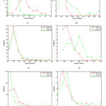Figure 7: The histogram of features of normal heart sound and murmur Click here to View Figure

From the histogram shown in fig. 7, it is noted that the separability among the features of both normal heart sound and murmur is not as much convincing. They exhibit overlap among features of both the classes. In the histogram of SR (fig. 7 (a)-(b)) and that of MF (fig. 7 (c)-(d)), the histogram equivalent to normal heart sound is somewhat lying sufficiently apart spatially from the histogram analogous to murmur. But the histogram of all other features, the separability among normal and murmur is very slight. Hence it has inferred that the features, namely SR and MF, has exhibited very limited overlapping, and the separability among them is also somewhat convincing.

The performance indicators of the system such as sensitivity, specificity, accuracy, positive predictive value (PPV) and negative predictive value (NPV) of all the features to categorize normal/murmur are also computed for the two datasets and are displayed in Table.3. The definitions and the mathematical formulations [23] are given as follows.

The sensitivity of a diagnostic test measures its capability to correctly distinguishing subjects with the disease condition. That implies, the percentage of sick people who are correctly identified sick. It is the proportion of true positives that are correctly recognized by the test, given by:

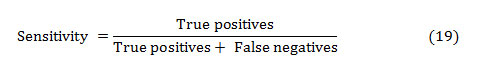
In general, True and False positive are the correctly and incorrectly identified subjects, respectively. The True and False negative are the correctly and incorrectly rejected subjects, respectively.

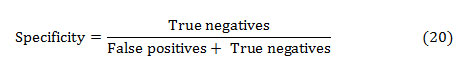
The specificity is the ability of a test to correctly identify subjects without the condition. That implies, the percentage of healthy people who are correctly identified as healthy. It is the proportion of true negatives that are correctly identified by the test:

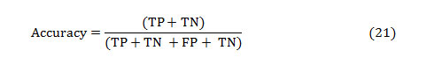
The accuracy of a test is its capacity to distinguish the normal and abnormal cases correctly. The accuracy can be estimated by calculating the proportion of true positive and true negative in all evaluated cases. The mathematical formulation is given as,

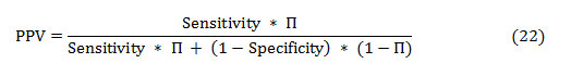
The PPV and NPV are the other two basic measures of diagnostic accuracy.  They are associated to sensitivity and specificity through a factor disease prevalence (Π). The PPV is the probability that the disease is present assumed a positive test result, and is given as:

Similarly, the NPV is the probability that the disease is absent given a negative test result, and is defined as:

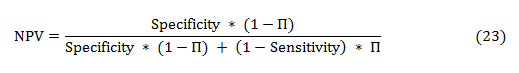
Table 3: Performance parameters of time domain features

Parameters	Spectral roll off		Median frequency		Spectral centroid		Dominant frequency		Spectral flux
	D1	D2	D1	D2	D1	D2	D1	D2	D1	D2
Accuracy	80.59	78.33	87.35	76.67	48.53	73.33	73.53	65	71.76	48.33
Sensitivity	80.59	80.00	87.65	63.33	48.24	66.67	66.47	53.33	65.88	23.33
Specificity	80.59	76.67	87.0	90.00	48.82	80.00	80.59	76.67	77.65	73.33
PPV	80.59	77.42	87.13	86.36	48.52	76.92	77.40	69.57	74.67	46.67
NPV	80.59	79.31	87.57	71.05	48.54	70.59	70.62	62.16	69.47	48.89

# D1- dataset 1, D2- dataset 2, all the parameters are expressed in percentage

By examining the performance parameters of all the features, the SR and MF are efficiently differentiating normal and murmur than that of other features. The SR offered a value of 80.59% for all the performance indicators. The accuracy, sensitivity, specificity, PPV, and NPV offered by SR to differentiate normal/murmur is 78.33,80.00,76.67, 77.42 and 79.31, respectively for dataset 2. The MF offers 87.35% accuracy, 87.65% sensitivity, 87 % specificity, 87.13 % PPV and 87.57 % NPV for dataset 1. For dataset 2 the parameters of MF are 76.67,63.33,90.00,86.36 and 71.05 percentage.  Hence, a method to detect the presence of murmur from the heart signal by using these features certainly may have its significance.

Conclusions

The significance of frequency domain features of PCG records for murmur detection was examined in this paper. For this, the statistical significance and feature separability of spectral features such as Dominant Frequency (DF), Spectral Centroid (SC), Spectral Flux (SF), Spectral using (SR) and Median Frequency (MF) was analyzed. The statistical significance of these frequency domain signatures was evaluated using Kolmogorov–Smirnov test, and the separability among the features were evaluated using the histogram. The values of Spectral roll off and median frequency relate to normal, and the murmur of dataset 1 differ with a ‘P’ value of 7.47×10^-29 and 1.73×10^-43, and that of dataset 2 is 6.17×10^-5 and 2.02×10^-4, respectively. The average accuracy offered by SR and MF to distinguish murmur and normal heart sound is 79.46% and 82.01 %, respectively. The method employing the frequency domain features can be utilized for the automated system meant for murmur detection. As a future deviation, the features can be given into various artificial classifiers and neural networks to check their ability to detect the murmur. The prospect of the ability of frequency domain features to separate the phenotypes of the murmur can also be studied as future expansion.

Acknowledgment

The authors would like to thank the people behind the Pascal heart sound database and Physionet heart sound database for providing the required PCG signals to test the proposed system.

Conflict of Interest

There is no conflict of interest.

 

Funding

This research received no specific grant from any funding agency in the public, commercial, or not-for-profit sectors.

References                                                                                            

1. World Health Organization. Cardiovascular diseases; 2017, URL https://www.who.int/en /news-room/fact-sheets/detail/cardiovascular-diseases-(cvds) (accessed:28.04.2020).
2. Samanta, A. Pathak, K. Mandana, and G. Saha, “Classification of coronary artery diseased and normal subjects using multi-channel phonocardiogram signal,” Biocybern. Biomed. Eng., vol.36, pp.426-443, Feb. 2019.
3. Surrel, A. Aminifar, F. Rincon, S. Murali, and D. Atienza, “Online Obstructive Sleep Apnea Detection on Medical Wearable Sensors,” IEEE Trans. Biomed. Circuits Syst., vol. 12, no. 4, pp. 762–773, Aug. 2018.
4. Wang et al., “Comparison of time-domain, frequency-domain and non-linear analysis for distinguishing congestive heart failure patients from normal sinus rhythm subjects,” Biomed. Signal Process. Control, vol. 42, pp. 30–36, Apr. 2018.
5. Isler, A. Narin, M. Ozer, and M. Perc, “Multi-stage classification of congestive heart failure based on short-term heart rate variability,” Chaos, Solitons & Fractals, vol. 118, pp. 145–151, January 2019.
6. S. Al-Zaiti, G. Pietrasik, M. G. Carey, M. Alhamaydeh, J. M. Canty, and J. A. Fallavollita, “The role of heart rate variability, heart rate turbulence, and deceleration capacity in predicting cause-specific mortality in chronic heart failure,” J. Electrocardiol., vol. 52, pp. 70–74, January 2019.
7. Hamidi, H. Ghassemian and M. Imani, Classification of heart sound signal using curve fitting and fractal dimension, Biomedical Signal Processing and Control, Vol.39, pp.351-359, Jan.2018.
8. Bozkurt, I. Germanakis, and Y. Stylianou, A study of time-frequency features for CNN-based automatic heart sound classification for pathology detection, Computers in Biology and Medicine, Vol.100, pp.132-143, Sept. 2018.
9. R. Thiyagaraja, R. Dantu, P. L. Shrestha and A. Chitnis, Mark A. Thompson, Pruthvi T. Anumandla, Tom Sarma and Siva Dantu, A novel heart-mobile interface for detection and classification of heart sounds, Biomedical Signal Processing, and Control, Vol.45, pp.313-324, Aug. 2018.
10. Chen, S. Zhao, S. Shao, and S. Zheng, “Non-invasive diagnosis methods of coronary disease based on wavelet denoising and sound analyzing,” Saudi J. Biol. Sci., vol. 24, no. 3, pp. 526–536, March 2017.
11. Kang, R. Doroshow, J. McConnaughey, and R. Shekhar, “Automated Identification of Innocent Still’s Murmur in Children,” in IEEE Transactions on Biomedical Engineering, Vol. 64, pp. 1326-1334, June 2017.
12. N. Varghese and K. I. Ramachandran, “Effective Heart Sound Segmentation and Murmur Classification Using Empirical Wavelet Transform and Instantaneous Phase for Electronic Stethoscope,” in IEEE Sensors Journal, Vol. 17, pp. 3861-3872, June 2017
13. A. Cha et al., “Time- and frequency-domain measures of heart rate variability predict cardiovascular outcome in patients with type 2 diabetes,” Diabetes Res. Clin. Pract., vol. 143, pp. 159–169, Sept.2018.
14. R. Sharma, A. Kumar, R. B. Pachori, and U. R. Acharya, “Accurate automated detection of congestive heart failure using eigenvalue decomposition based features extracted from HRV signals,” Biocybern. Biomed. Eng., vol. 39, no. 2, pp. 312–327, June 2019.
15. M. Fahad, M. U. G. Khan, T. Saba, A. Rahman and S. Iqbal, Microscopic abnormality classification of cardiac murmurs using ANFIS and HMM, Vol.81, pp.449-457, May 2018.
16. F. Maddams, “The Scope and Limitations of Curve Fitting,” Appl. Spectrosc., vol. 34, no. 3, pp. 245–267, May 1980.
17. G. Gutierrez et al. “Sex Differences in Comorbidity, Therapy, and Health Services’ Use of Heart Failure in Spain: Evidence from Real-World Data.” International journal of environmental research and public health, Vol. 17, pp.1-13, Mar. 2020.
18. Bentley, G. Nordehn, M. Coimbra, S. Mannor, G. Rita, the pascal classifying heart sounds challenge, sponsored by PASCAL, 2011.
19. Classification of Normal/Abnormal Heart Sound Recordings, the PhysioNet/Computing in Cardiology Challenge,2016.
20. Joy et al., “The diagnostic feasibility of median frequency of lung sounds,” 2015 IEEE International Conference on Electronics, Computing and Communication Technologies (CONNECT), Bangalore, 2015, pp. 1-6.
21. Joseph, N.S. Haider and R. Periyasami, “An investigation on the statistical significance of spectral signatures of lung sounds,” Biomedical Research, Vol.28, pp. 2801-2810, Jan 2017.
22. F. Fuentes, M.R. Lopez, O. Sergiyenko, F.F.G. Navarro, J.R. Castillo, D.H. Balbuena, and J.C.R. Quinonez, “Combined application of power spectrum centroid and support vector machines for measurement improvement in optical scanning systems,” Signal Processing, Vol. 98, pp. 37-51, May 2014.
23. Wong and G. H. Lim, “Measures of Diagnostic Accuracy: Sensitivity, Specificity, PPV and NPV,” Proc. Singapore Healthc., Vol. 20, pp. 316–318, Nov.2011.

 

(Visited 1,028 times, 1 visits today)