S. M. Nazia Fathima, R. Tamil Selvi and M. Parisa Beham

Department of Electronics and Communication Engineering, Sethu Institute of Technology, Tamil Nadu, India-626115

Corresponding Author E-mail: naziafathima@sethu.ac.in

DOI : https://dx.doi.org/10.13005/bpj/1822

Abstract

Biomedical engineering is one of the promising disciplines in engineering that deals with technology advancement in human health. Osteoporosis is a common metabolic disease categorized by decreased bone mass and increased liability to fractures. Bone densitometry is a broad term comprising the art and science of measuring the bone mineral content (BMC) and bone mineral density (BMD) of particular skeletal sites or the whole body. There are various methods to measure bone mineral density which differs based on the differential absorption of ionizing radiation or the sound waves. The methods are SPA (Single Photon Absorptiometry), DPA (Dual Photon Absorptiometry), SEXA (Single Energy X ray Absorptiometry), DEXA (Dual Energy X ray Absorptiometry), QCT (Quantitative Computed Tomography), QUS (Quantitative Ultra Sound) and RA (Radiographic absorptiometry).  The DEXA test can measure the whole body but usually the lower spine and hips. A major disadvantage of DEXA is that currently there is a lack of standardization in bone and soft tissue measurements. Furthermore, for a given manufacturer, results may vary by the model of the instrument, the mode of operation or the version of the software used to analyze the data. In addition to that, DEXA scan images are only for the confirmation of correct positioning of the patient and correct placement of the regions of interest (ROI). Motivated by the above issues, this paper can pave a way for analysis in the measurement of BMD, measurement of T-score, and Z-score from the DEXA scan images. This proposed methodology includes segmentation algorithms such as k means clustering & mean –shift algorithm and comparison of the accuracy of algorithms. Also in addition, a novel mathematical analysis is also proposed to measure the T–score values in DEXA images with a new parameter ‘S’ from BMD values in order to detect the osteoporosis condition accurately.

Keywords

Bone Mineral Density (BMD); Osteoporosis and T Score; Segmentation

Download this article as: 

Copy the following to cite this article: Fathima S. M. N, Tamil Selvi R, Beham M. P. Assessment of BMD and Statistical Analysis for Osteoporosis Detection. Biomed Pharmacol J 2019;12(4).

Copy the following to cite this URL: Fathima S. M. N, Tamil Selvi R, Beham M. P. Assessment of BMD and Statistical Analysis for Osteoporosis Detection. Biomed Pharmacol J 2019;12(4). Available from: https://bit.ly/2NqlDJQ

Introduction

Measuring the density of the bone plays a vital role in the analysis of the human bone health. This is a very important feature in the field of medical image processing. The diagnosis and effective treatment directly lies in the statistical analysis and models of the bone structure[1].There are many scanning methods available to measure BMD and detect osteoporosis condition. Among those methods, DEXA is the recent method used in the medical field for the analysis of BMD.   The starting point of the DEXA scan has big olden times. To detect the fracture risk of bone in major areas such as AP Spine, Left femur and Right femur, scanners like X-ray, CT scan were used. The bone density scan was initiated by Dr. John R Cameron. The present DEXA scan principle is that the energy of X-ray beams are passed through the bones and are absorbed and the division that is not riveted is perceived on the other side of the body. If the bone is denser, then additional energy will be fascinated and less energy will be sensed effectively. In 1980s, the most expensive and superior radioactive sources have been outdated by Single X-ray Absorptiometry (SXA) and Dual Energy X-ray Absorptiometry. DEXA is dependent on the Age factor (i.e.) to estimate the BMD of the bone and also we need to know the T-Score, Z-Score and the age of the patient to detect whether the patient is suffering from Osteoporosis or Osteopenia or Normal.

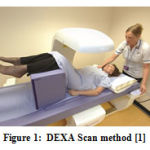Figure 1:  DEXA Scan method [1] Click here to view figure

Fig.1 shows the positioning and measuring method in the DEXA scan image. In a statistics taken in India for the women aged 30 to 60, BMD were very much low with high risk of Osteopenia and Osteoporosis with the assumption that due to lack of nutrition. In women approximately, 80% forearm, 70% hip and 58% spine fractures occurs very often. On the whole 61% of osteoporotic fractures occur in women. About 75% of hip, spine and forearm fracture occurs among 65 years old or above. Fig. 2 shows the sample Dexa images.

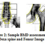Figure 2: Sample BMD assessment in Dexa spine and Femur Image Click here to view figure

World health organization (WHO) defines the BMD plot T score values for human beings.

For Normal condition

T-score at or above -1 SD (Standard Deviation)

For Osteopenia condition

T-score between -1 and -2.5 SD

For Osteoporosis condition

T-score at or below -2.5 SD. [2]

In order to recognize more about bone density, several methods have been initiated by the researchers for structuring bone and the relationship between bones mass for the complete analysis of the bone structure. Even though a lot of methods are available for estimation of BMD, it is better to obtain a gold standard method for the effective BMD measurement apart from normal scores.

In this proposed work, an innovative method for BMD analysis is derived. Also we propose a formative and mathematical analysis to estimate an index that indicates the connectivity of bone mineral components and structural view of the image. The proposed work involves the estimation of the novel index based on the study of the entropy value of the Dexa scan images .A novel parameter called S-Measure is predicted for the bone connectivity based on the segmentation method and entropy. Also we have estimated S_T corresponding to T score of the scan images. Involving the estimation of maximum entropy, the obtained results are validated with the clinical reports of the DEXA images to detect the osteoporosis.

The paper is organized as follows: Section 1 explains the introduction about the DEXA and history of BMD. Section 2 explains the technical background of the DEXA scan images. Section 3 explains the importance of k means clustering algorithm and its procedure in segmentation process. Section 4 details about the various steps involved in the mean shift algorithm for segmentation. Section 5 explains the statistical analysis of the algorithm and evaluation of S-parameter based on the entropy value. Section 6 concludes the proposed work.

Technical Background

Bone mineral density is the amount of minerals content exists in bone tissue. This idea depend on mass calculation per volume of bone, still it is calculated by proxy according to the optical density per square centimetre of surface of bone on Imaging.. In present medical field, BMD is measured using DEXA which provides better results in detection of osteoporosis. The normal average BMD in males is about 3:88 g/cm² and in females are 2:90 g/cm². The range of BMD in the forearm is from 700 to 800 g/cm² and in the spine region is 1000 to 1200 g/cm². The density of hard bone is a constant number of 1900 kg/m³ [2].

In DEXA scan, the major scan detector regions include hip bone, spine–lumbar and whole body. Fig. 3 shows a picture of a femur that was scanned by a DEXA scan and a BMD plot report. In general, after the scanning of the bone image to the system, an automatic algorithm runs and calculate the required scores for BMD calculation. The T-score is the standard deviation (SD) of the patient’s BMD above or below the mean for the Young-Adult normal reference population. The Z-score is the SD of the patient’s BMD above or below the mean of the Age-Matched population [2].

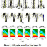Figure 3(a): Lumbar spine Dexa Scan Image (b) Femur Dexa Scan Image (c) BMD Plot Image Click here to view figure

K – means Clustering Algorithm

Image segmentation is a very important process to differentiate the similar and dissimilar characteristics in an image. In bone images, scanning involves the departure of bone structure from other regions such as muscle and background. This is a very important challenge in bone X-ray imaging. Region of interest (ROI) and crack, fracture, bone mineral density (BMD) estimation and deformation is predicted by the segmentation of bone region. However, conventional segmentation methods don’t produce acceptable results on bone images. There are various segmentation methods available such as measurement of space clustering, region growing, split-and-merge segmentation, edge detection, active contours, etc. Among the various algorithms, K-means clustering is one of the greenest unsupervised classification practices. The method is a very simpler method in the unsupervised learning algorithm; hence it is a popular method. The main dissimilarities between a supervised classifier and an unsupervised classifier is that a training data set with known class labels is compulsory for the former to train the classification rule, whereas such a training data set and the awareness of the class labels in the data set are not compulsory for the latter.

Portrayal of the Algorithm

The k-means clustering algorithm walls a specified data set into ‘k’ mutually exclusive clusters. By the method of divider, the sum of the distances between data and the equivalent cluster centroid is decreased. The expressed distance ratio between two data points is reserved as a measure of similarity. The given data set determines the number of distance measures. A number of distance measures can be used depending on the data. Various distance measures like Minkowski distance, Euclidean distance and Mahalanobis distance are available for measuring the distance between the pixels. In our method, the standard Euclidean distance is depicted as the distance measure.

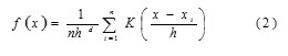
In Mathematical analysis, given a set of data vectors X = [x1, …, xn] where n is the number of observations. The k means clustering algorithm clusters the data into k clusters with the target at diminishing an objective function, a squared error function. The objective function, when the Euclidean distance is expressed as the distance measure in this proposed method, then clearly given as c_j

where c_j is the j-th cluster and µj, is the centroid of the cluster cj . Therefore, the k-means clustering algorithm is an iterative algorithm that finds a suitable partition which minimizes the sum squared error. The algorithm begins with the initialization of k cluster centroids.

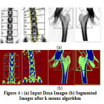Figure 4 (a): Input Dexa Images (b) Segmented Images after k means algorithm Click here to view figure

A simple method is to initialize the problem by randomly select ‘k’ data points from the given data. The remaining data points are classified into the k clusters by distance. The centroids are then updated by computing the centroid in the k clusters [3].

The proposed k means segmentation involves the formation of two clusters as background and bone tissue. Fig. 4(a) shows the input Dexa images. The results are based on the initial seed and the total number of clusters. For our proposed algorithm, two clusters are defined, one for the soft tissue and other for the bone tissue. The above results show that the fig. 4b shows the segmented results after k means clustering algorithm. The Euclidean distance establishes the distance between each data object and the cluster centres. The proposed method can be used for better segmentation and classification.

Mean shift clustering Algorithm

Apart from the k means algorithm, we are interested in another segmentation algorithm such as mean shift segmentation algorithm. The mean shift algorithm is a nonparametric clustering technique which does not need earlier information of the figure of clusters, and does not limit the shape of the clusters. In a d-dimensional space R_d, with  n data points x_i , i = 1, …, n , the multivariate kernel density estimate obtained with kernel K(x) and window radius h is

The kernel k(x) is defined by the radically symmetric kernels,

where c_k,d is a normalization constant which guarantees K(x) integrates to 1. The modes of the density function are located at the zeros of the gradient function.

The gradient of the density estimator is

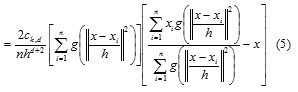
where g(s) = −k₀(s). The first term is proportional to the density estimate at x computed with kernel G(x) =

C_g, _dg(||x||²) and the second term

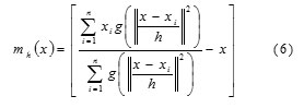
m_h(x) is the mean shift. The mean shift vector always points toward the direction of the maximum increase in the density. The mean shift process, attained by successive calculation of the mean shift vector m_h(x^t),the transform of the window x^t+1 = x^t +m_h(x^t) is definite to converge to a point where the gradient of density function is zero [4]. The Fig. 5 (a), (b) and (c) shows the spine, left and right femur images respectively. Fig. 5 (d), (e) and (f) shows the mean shift segmented image of spine, left and right femur respectively.

The results show that according to the gray level distribution, the ROI is segmented distinctly. The segmented result depends on the mean shift mode. The mean shift technique is encompassing of two fundamental steps

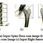Figure 5: (a) Input Spine Dexa scan image (b) Input left femur Dexa scan Image (c) Input Right femur Dexa scan. Click here to view figure

 

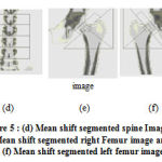Figure 5: (d) Mean shift segmented spine Image, (e) Mean shift segmented right Femur image and (f) Mean shift segmented left femur image. Click here to view figure

(i) A mean shift filtering of the original image data and (ii) A succeeding clustering of the filtered data points. Two parameters related to the bandwidth (radii of the kernel) are involved in the mean shift filtering stage the spatial (h_s) and colour (h_r) features.

Mathematical analysis of the proposed method

From the above segmented results, the entropy of the segmented image is estimated to validate the T score and Z score. Also the BMD is measured using the standard equation with respect to the Mean Gray Levels (MGL) [5].

The ROI’s with various regions were defined in the bone for the BMD measurement. On every image, the mean grey levels were measured in each defined ROI’s. A linear regression algorithm was used to find out the correlation between the MGL values and the corresponding BMD values. It was found that there was a statistically significant (p<0.001) correlation between these two values. In the attained linear regression equation, the calculated mean MGL on various ROI’s were replaced independently and their equivalent BMD values were estimated [5].

where       X=  Mean (MGL)+SD

and SD is the Standard Deviation

The estimated BMD value is compared with the Database BMD value obtained from the Hospital. From the linear regression equation, the BMD values are calculated for the segmented output of k means clustering and mean shift segmentation algorithm. Table 1 shows the BMD values of Anti-Posterior Spine measured by using linear regression Equation with mean gray levels. Table 2 shows the BMD values of left femur measured by using linear regression Equation with mean gray levels. Table 3 shows the BMD values of right femur measured by using linear regression Equation with mean gray levels.

Table 1: BMD values of Anti-Posterior Spine

ID	Anti-Posterior Spine(BMD) g/cm2
	Given database value	K means	Mean shift
1	0.99	0.9690	1.0253
2	0.967	0.9547	1.0154
3	1.025	0.9638	1.0279
4	1.085	0.9628	1.0204
5	1.029	0.9686	1.0269

 

Table 2: BMD values of Left Femur Bone

ID	Left Femur (BMD) g/cm2
	Given database value	K means	Mean shift
1	0.923	0.9730	1.0385
2	0.791	0.9602	1.0283
3	0.976	0.9682	1.0346
4	1.126	0.9707	1.0397
5	0.863	0.9653	1.0350

 

Table 3: BMD values of Right Femur Bone

ID	Right Femur (BMD) g/cm2
	Given database value	K means	Mean shift
1	0.887	0.9730	1.0397
2	0.796	0.9702	1.0369
3	1.015	0.9648	1.0328
4	1.12	0.9674	1.0351
5	0.883	0.9616	1.0344

From the above tabulated results, it is analyzed that the obtained BMD values for mean shift algorithm gives better results when compared with the Clinical database value. The accuracy is more than 95 % of the clinical Database values. The table values shows that the Mean shift segmented BMD value is approximately equal to the database clinical value.

Maximum Entropy value and Estimation of S parameter related to T Score and Z score Value

The entropy of an image can be explained as an assessment of the ambiguity connected with a random variable and it compute, in the sense of an accepted value, the information enclosed in a message. Entropy of an image E depicts a scalar value demonstrating the entropy of greyscale image I. Entropy is a numerical measure of randomness that can be used to exemplify the texture of the input image.

Entropy is defined as

where p contains the histogram counts [6].

The maximum Entropy value of the segmented image and the original image is calculated by the conventional definition of entropy.

Two entropy values are calculated as

entropy of the background (s_max) and

entropy of the bone tissue(s_min)

The two entropy calculated values are denoted as S_min and S_max. The S parameter is denoted as

where the parameter Ω is selected as 0.25. From the Eqn.(9) the S parameter values are estimated for the mean shift segmented images.

Standard T score value is represented in the clinical representation as

where BMD is the Bone Mineral Density  and    is the Standard Deviation. Using this Eqn.(10), clinical T score value is estimated.

The proposed S_T score value is predicted as

Table 4 and 5 describes the estimated BMD and S_T score by the proposed statistical method and validates the results with the clinical database.

Table 4: T-score values based on S –parameter and clinical Database

Unique Id	Database T-Score value	Calculated S_T score value
1	-1.6	-1.19
2	-1.8	-1.27
3	1	-1.17
4	-0.8	-1.23
5	-1.3	-1.18

 

Table 5: Estimated BMD and T-score value and the kind of Risk derived from WHO standard

Patient Id	Part	BMD	T-Score	Kind of Risk
001	Ap Spine	1.0253	-0.1	Normal
	Left Femur	1.0385	-1.4	Osteopenia
	Right Femur	1.0397	-2.9	Osteoporosis
002	Ap Spine	1.0154	-2.6	Osteoporosis
	Left Femur	1.0283	-2	Osteopenia
	Right Femur	1.0369	-0.9	Normal

Conclusion

We measured a new T -Score value for bone density based on S parameter entropy in DEXA images.The developed work determines the variations in the average intensity of the bone to determine the BMD. A new database is created and the T score values that are calculated based on the entropy values are validated with the clinical report. The risk of fracture or whether it is osteopenia or osteoporosis is found out by our proposed method using classification of WHO.

References

1. Yong Jun Choi, “  Dual-Energy X-Ray Absorptiometry: Beyond Bone Mineral Density Determination”, Endocrinology and Metabolism,Vol 31,2016,pp.25-30
2. Li Chen and V. B. Surya Prasath, “Measuring Bone Density Connectivity Using Dual Energy X-Ray Absorptiometry Images”, International Journal of Fuzzy Logic and Intelligent Systems Vol. 17, No. 4, , pp. 235-244,2017.
3. Gobert N. Lee and Hiroshi Fujita, “K-means clustering for classifying unlabelled MRI data”, Digital Image Computing Techniques and Applications,pp.92-98,2007
4. Miguel ´ A. Carreira-Perpinan “A review of mean-shift algorithms for clustering”, CRC Handbook of Cluster Analysis, 2015,pp.1-28
5. C Aroba Sahaya Ligesh, N Shanker and C C Glueer, “Estimation of Bone Mineral Density from the Digital Image of the Calcanium Bone”, IEEE proceedings on ICECT,2011.
6. H.S.Prasantha,.Shashidhara.H.L, .N.B.Murthy and Madhavi Lata.G, “Medical Image Segmentation”, International Journal on Computer Science and Engineering Vol. 02, No. 04, pp. 1209-1218, 2010.

(Visited 1,656 times, 1 visits today)