D. Stalin David

Department of CSE, PSN College of Engineering and Technology, Tirunelveli, 627011, India.

Corresponding Author E-mail: sdstalindavid707@gmail.com

DOI : https://dx.doi.org/10.13005/bpj/1720

Abstract

The most common type of brain tumor known as Meningioma arises from the meninges and encloses the spine and the brain inside the skull. It accounts for 30% of all types of brain tumor. Meningioma’s can occur in many parts of the brain and accordingly it is named. In this paper, we propose Meningioma brain tumor classification system using MRI image is developed . Firstly, based on the characteristics of MRI image and Chan-Vese model, we use multiphase level set method to get the interesting region. Therefore, we obtain two matrixes, in which one contains the whole cell's boundary, and the other contains the boundary of some cells. Secondly, with respect to the cells' boundary, it is necessary to further processing, which ensures the boundary of some cells is a discrete region. Mathematical Morphology brings a fancy result during the discrete processing. At last, we consider every discrete region according to the tumor's features to judge whether a tumor appears in the image or not. Our method has a desirable performance in the presence of common tumors. For some non-convex tumors, we utilized a traditional way (SVM and LBP) as a second processing, which increased the coverage and accuracy. Experiments show that our method has a high coverage without any learning-based classifiers for most common tumors, which saves a lot time and reduces a lot workload. Therefore, the proposed method has a good practical application for assisting physicians in detecting Meningiom tumors using MRI images.

Keywords

Gaussian High-Pass Filtering; Multilevel Thresholding; Parasagittal Meningioma Tumor; Skull Stripping

Download this article as: 

Copy the following to cite this article: David D. S. Parasagittal Meningioma Brain Tumor Classification System Based on Mri Images and Multi Phase Level Set Formulation. Biomed Pharmacol J 2019;12(2).

Copy the following to cite this URL: David D. S. Parasagittal Meningioma Brain Tumor Classification System Based on Mri Images and Multi Phase Level Set Formulation. Biomed Pharmacol J 2019;12(2). Available from: https://bit.ly/2GeBOpZ

Introduction

Our brain is a complex integrative network where information is continuously processed and shared between structurally and functionally interconnected regions. Functional magnetic resonance imaging (fMRI) indirectly measures such brain activities by detecting relative alterations in blood oxy- gen level. For the past three decades, most studies have been carried out focusing on localization of neural activities associated with a variety of cognitive, sensory and motor tasks. Recent developments in functional neuro imaging have shifted the research focus to investigating and interpreting functional interactions between different brain regions.^1-3 Study of interactions between brain regions (i.e., brain connectivity) has the potential to provide insights into neural activity related to human behavior and about the alterations of these connectivity’s in neurodegenerative diseases.⁴ While connectivity studies can be targeted at exploring task-related interactions among brain regions, similar studies can be carried out on resting-state fMRI as well, investigating the spontaneous interaction between brain regions without the subject concentrating on a specific task. The resting state connectivity studies are particularly useful when it is difficult for the subject (e.g., due to dementia) to actively engage in sensory, motor or cognitive tasks.⁵

Brain is the major organ of our body that is composed of nerve cells and tissues that control the main activities of the entire body like movement of muscles, breathing and our senses. Tumor also referred to as neoplasm, are a collection of atypical tissues or cells that can have a rapid growth than normal cells and can be life threatening. Under the skull we have three layers of membranes, Dura Mater, Arachnoid Mater and the Pia Mater, collectively called meninges, which act as a protective tissue for the brain and the spinal cord. Tumor that originates in the meninges are known as Meningioma Tumor. Depending on the location, there are different types of Meningioma’s. They are: Convexity Meningioma, Falcine Meningioma, Parasagittal Meningioma, Intraventricular Meningioma, Skull base Meningioma, Sphenoid wing Meningioma, Olfactory groove Meningioma, Petrous Meningioma, Suprasellar Meningioma and Recurrent Meningioma.^6-8 The naming of the Meningioma Tumors is based on the location it occupies in the brain. The growth rate of Meningioma Tumors are very slow and therefore often people suffering from Meningioma Tumors are unaware that they are having the tumor in the brain. In many cases patients come to know about it due to sudden critical seizure and numbness in their hands or legs. Depending on the position of the tumor in the brain certain parts of the body are affected. For example, a person having Parasagittal Meningioma tumor in the left side of the brain will find difficulty on their right hand and right leg movement. They will feel numbness, shivering on their right side and will also find difficult in seeing. When tumor exist on the left side of the brain, part of the brain controlling emotions are also strained.

Our Main Focus in this paper is in the extraction of Parasagittal Meningioma Tumor in the Brain from images acquired from digital imaging technologies like CT scan, MRI, etc. Tumors in the brain that are adjacent to the convexity dura and the falx and are associated with the superior sagittal sinus are known as Parasagittal Meningioma Tumor. Based on their association with sagittal sinus, the parasagittal meningioma tumors are classified into three categories: Anterior, Middle and Posterior. The anterior third spreads from the cristi galli to the coronal suture, the middle third of the sinus spreads from the coronal to lambdoid suture and the posterior third spreads from the lambdoid suture to the torcula.⁹ The occurrence rate for parasagittal meningioma is 16.8% to 25.6 %. Familiar symptoms are headache, seizures, personality changes and motor weakness. Parasagittal Meningioma tumor can be divided into three types. Type 1, where the tumor is attached to the outer surface of the superior sagittal sinus. Type 2, where the tumor pervade the superior sagittal sinus although the lumen remains patent and type 3 where the tumor invades and cause the occlusion of superior sagittal sinus. Since the superior sagittal sinus allows blood to drain and also helps in venous circulation of the cerebrospinal fluid, it is important to protect the superior sagittal sinus while operating parasagittal meningioma tumor as injuring the sinus increases the mortality rate.^10-13

Image processing techniques in diagnosing or analyzing biomedical issues are trending and rapidly growing due its ease, accuracy, cost effectiveness and less time requirement in detecting a disease from MRI scanned images as well as other form of images gained from medical imaging technologies. In this paper we have proposed an algorithm that uses many image processing techniques in MATLAB like filtering to reduce noise and sharpen the image. The algorithm determines the threshold value from histogram and uses skull stripping method and other processing techniques in MATLAB to extract Parasagittal Meningioma tumor in Brain. We used the algorithm in 50 MRI images that included both the presence and absence of parasagittal meningioma tumor. The algorithm demonstrated its efficiency in extracting the tumor accurately and plotting the region boundaries of the tumor. If the image contains any tumor other than parasagittal tumor, the algorithm efficiently delivers the result as the absence of parasagittal meningioma tumor.

Proposed Brain Tumor Classification System

In our algorithm we have used Gaussian High Pass Filtering, Histogram, Skull Stripping Method, Multilevel Thresholding, level set techniques to extract Parasagittal Meningioma Tumor in the Brain from MRI Images. Segmentation has also been used widely that helped in differentiating the parts of the image that are found abnormal. Proposed algorithm has been tried in 50 images including images containing tumors and images that are void of tumors. We have also tried with images that contained tumor but not Parasagittal Meningioma Tumor.

Preprocessing

Gray scale images help in distinct identification of edges which in a way helps in proper detection of the tumor region. Use of gray scale images reduces the complexity of the code and helps in proper minimization of time in differentiating the tumor region from the normal parts in the brain. Gaussian high-pass filtering provides intricate information from the image by sharpening the image and enhancing minute details of the image. On the other hand we don’t receive this information using low pass filtering. Hence Gaussian high-pass filtering helps in extracting the boundaries of the tumor region and to get accurate results.

Level Set Functions

In the past decade, the level set method, originally used as numerical technique for tracking interfaces and shapes,¹⁹ has been increasingly applied to image segmentation,^18,22–26 In the level set method, contours or surfaces are represented by implicit functions which usually called a level set function and its zero level set. With the implicit function, the image segmentation problem turns to solve the energy equation in a principled way based on well-established mathematical theories, including calculus of variations and partial differential equations (PDE). In,^18,22 the level set method was introduced independently in the active contour models for image segmentation. Early active contour models are formulated in terms of a dynamic parametric contour C(s; t) → R² with ‘s’ belongs to [0; 1] parameterizes the points in the contour, t belongs to [0; 1) is a temporal variable. The curve evolution is expressed as the following eqn.

where F, controling the motion of the contour is the speed function, and N is the inward normal vector to the curve. We can rewrite the above eqn to a level set formulation by embedding the dynamic contour C(s; t) as the zero level set of a higher dimensional function (x; y; t). Assuming that the embedding function (x; y; t) takes negative values inside the zero level contour and positive values outside, such as 2-Dimension shown as in Fig.1

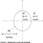Figure 1: Dimension Level set Example.   Click here to view figure

 

The inward normal vector can be expressed as

where ∇ is the gradient operator. Then, equation can be expressed as the following partial differential equation (PDE)

which is referred to as a level set evolution equation. The level set formulation can implicit represent the active contour which is called geometric active contour model. In,³⁶ some parametric active contours and their corresponding level set formulations are defined.

Although the level set method is too cumbersome in computational complexity, it still has a unique advantage: first of all, the coordinate system for the level set method of the given PDE is fixed, so it is a no parameter method, secondly, a topology change may occurs for the curve during the evolution process, for the level set method, the whole curve movement is embedded in the high-dimensional surface motion, so the curve on the topology changes are same embedded in the high-dimensional surface motion, thirdly, the segmentation accuracy of the level set can reach sub-pixel, and the medical images require a class of high precision, so the level set has a wide range of applications, shows in Fig.2.

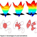Figure 2: Advantages of Level set method.   Click here to view figure

 

Multiphase Level Set Formulation

According to the two clues, lumen and illumination high-light, we processed MRI images with histogram equilibrium to enhance image contrast as the first step. Obviously there are others image manipulation enhanced algorithms, such as linear contrast broadening, retinex model and so on. However all the transformation must be homeomoriphic, since related research³⁰ showed that in a image, the shape information of objectives was represented through levelset of the image, in another words the shape information of objectives was included in the isolux lines of image. In this paper, we adopted histogram equilibrium to improve image contrast. It makes the illumination of tumors prominent.

Allow for the whole cell’s boundary, which imbedding in the black background. We adopt multiphase level set formulation, in theory, two boundary can indicate 4 regions, according to analyzing, that the region of interest is whole included in the bigger boundary, so we use two boundary represent 3 regions in this work. Moreover, this method shows a desirable performance in the presence of intensity in homogeneities for both synthetic and real images.¹⁷ Therefore, the method is good at intensity in homogeneities, suitable for the illumination high-light. Simultaneously, the method is appropriate for another clue, the lumen highlight. We consider the three-phase case: the MRI image domain is segmented into three disjoint regions 1, 2 and 3. Meanwhile, two level set function 1 and 2 is used to define the three regions.

Mathematical Morphology

Mathematical morphology is based on the collection theory, topology and random function of the geometric structure analysis and processing technology. Mathematical morphology is most commonly used for digital images, but can also be used for graphics, surface grids, entities, and many other spatial structures. Mathematical morphology introduces the concept of topological and geometric continuous spaces in continuous and discrete spaces, such as size, shape, convexity, connectivity and geodesic distance. Mathematical morphology is also the basis of morphological image processing, which consists of a set of operators according to the above characteristics of the image composition. Basic morphological operators include expansion, corrosion, opening and closing operations. Mathematical morphology from the initial processing of binary images, and gradually developed to deal with grayscale image color images. The opening of A by B is obtained by the erosion of A by B, followed by dilation of the resulting image by B.

A° B = (A Θ B) ⊕ B

which means that it is the locus of translations of the structuring element B inside the image A. In the sense the opening opens up holes that are near (with respect to the size of the structuring element) a boundary, and removes small object protuberances(opening makes the sharp edges be smoothed). Moreover, the opening is able to break the weak connection of touching-cell, in another words it makes some regions of interest discrete, which is what we wanted and it will be easier for the next phase. That’s why we choose the concise and effective opening in this work. Of course, there are some other complicated but technical way  to deal with touching-cell.

Classification

Statistical classification involves predicting an output for a given input. Algorithms for classification contain a training set with a set of attributes and their relevant outputs. The respective outputs can also be termed as output predictors. Classifier algorithms determine relationships between the set of attributes to predict a possible outcome. Once the relation is defined, the classifier is said to be trained. When the data from the testing set is fed to the trained system, the system analyzes the incoming data and predicts the class output. The algorithm efficiency is evaluated based on the prediction accuracy of the classifier algorithm.^22-24 In this work, hybrid RBF kernel based SVM classifiers are investigated to classify the normal and glaucomatous images.

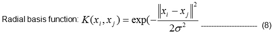
SVM is a supervised learning algorithm consisting of generalization theory and kernel functions.²⁵ It is used for classification and regression studies. SVM classifier can be divided into two types based on the data distribution. If the data is linearly separable, it is termed as a linear SVM classifier. If the data is linearly inseparable, then kernel functions (radial-basis function, polynomial function of order 1, order 2 and order 3) are used to map the linearly inseparable data to a higher dimensional feature space where the data is presumed to be linearly separable.

The kernel function can directly compute the dot product in the higher dimensional space.

Kernel- based Lagrange multipliers is given by Eqn.

Classification

Statistical classification involves predicting an output for a given input. Algorithms for classification contain a training set with a set of attributes and their relevant outputs. The respective outputs can also be termed as output predictors. Classifier algorithms determine relationships between the set of attributes to predict a possible outcome. Once the relation is defined, the classifier is said to be trained. When the data from the testing set is fed to the trained system, the system analyzes the incoming data and predicts the class output. The algorithm efficiency is evaluated based on the prediction accuracy of the classifier algorithm.^22-24 In this work, hybrid RBF kernel based SVM classifiers are investigated to classify the normal and glaucomatous images.

SVM is a supervised learning algorithm consisting of generalization theory and kernel functions.²⁵ It is used for classification and regression studies. SVM classifier can be divided into two types based on the data distribution. If the data is linearly separable, it is termed as a linear SVM classifier. If the data is linearly inseparable, then kernel functions (radial-basis function, polynomial function of order 1, order 2 and order 3) are used to map the linearly inseparable data to a higher dimensional feature space where the data is presumed to be linearly separable.

The kernel function can directly compute the dot product in the higher dimensional space.

Kernel- based Lagrange multipliers is given by Eqn (7),

α_i ≥ O∀_i

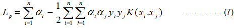
Minimize L_p with respect to w, b and maximize with respect to α_i.

There are several common kernel functions are given in Eqn(8), namely,

Linear: y_i⋅ y_j,

Polynomial of degree d: (y_i⋅ y_j + 1)^d,

Let K₁ (RBF) and k₂ (RBF) be kernels over

and k_a be a kernel over R^{P χ} R^P Let function

The pair of RBF kernels based designs are signified in Eqns (9).

k(x,y) = k₁ (x,y) + k₂ (x,y) is a kernel

k(x,y) = k₁ (x,y) k₂ (x,y) is a kernel ——–(9)

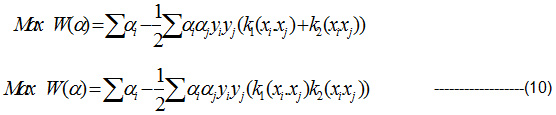
Substitute the Eqn (9) in Lagrange multiplier and get the projected Pair of RBF kernel. It is given in Eqn(10):

Discussion and Experimental Results

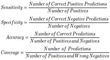
For performance evaluation of the proposed algorithm, we use an experimental data set which contains 33 tumor images from 6 pathological cases with different tumor appearances and 100 normal images from 6 normal pathological cases. These images are obtained from a hospital. In a real situation, most frame in the video is normal pathological cases, so we use a few number of tumor images and a large number of normal images. In this case, 23 normal samples and 80 tumor samples are used as the training set. To test the performance of the proposed method, each image is manually labeled as a positive sample (tumor image) or a negative one (normal image) to create the standard. All this just to train the classifier, the classifier just used for the non-convex images, which means we first use the multiphase level set method deal with all the images and do the judgement, when there is a result shows it’s a normal image, it’s time to use the SVM classifier do the quadrature detection. At last, the average recognition rates are used to demonstrate the performance of the proposed method. Success of the MRI image identification is measured due to its sensitivity, specificity, accuracy and coverage which can be explained as follows.

The sensitivity represented the availability of algorithm, the low sensitivity showed that there are many real tumor images can not be detected, so the coverage can not be good, in another words, there are some missing detection in the actual medical treatment, which contrary to the essence of medical. The Specificity was used to measure the number of misjudgment, which means the high specificity will further reduce the burden of clinicians, after all, all the tumor images predicted needed another check by clinicians. Actually, both the high sensitivity and high specificity shows the high coverage. As for the accuracy revealed the general performance of the method. The higher coverage provides higher practicability, the location of algorithm was assisted detection, it is used to reduce clinicians’ workload, so the higher coverage means the results including more real tumor images and filter out many normal images.

The performance of the proposed level set method based on region-model and mathematical morphology for automatic tumor detection is shown as in Table 1, independently. Ac-cording to the results, the utmost sensitivity is 72.7% when the radius of opening equals 8, that expressed we can detect the tumor as much as possible, on the contrary the bigger radius caused a large numbers of misjudgment, which leaded to the specificity so low, 50% means that just a half normal can be filtered out and it’s still a heavy workload for clinicians. Taking into consideration various factors, we let the radius of opening equals 5 in this work and the later analysing. When the radius of opening equals 5, it makes most weak connection broken between cells and keep the shape of most boundaries, simultaneously. Also, the results showed as in Table 1 indicate the best specificity and accuracy when the radius is taken as 5. On the other hand, most threshold is a empirical value when we made our decision and there is no standard in history, so the results might have a little difference if the threshold changed. From a practical sense, the results in Table 1 can not be used in the actual medical treatment, although the level set method is another way no one used up to now in wce images and it’s a no-training way, which will save some time. It’s necessary to do the quadrature detection to enhance sensitivity, specificity, accuracy and coverage, so we judged those non-convex images again by means of support vector machine (SVM) based on discrete wavelet transform (DWT) and uniform local binary pattern (ULBP). The performance of the proposed level set method and SVM is shown in Table 2. Both the high sensitivity(90.9%) and specificity(85%) expressed the high coverage(93.75%),so it will be feasible in the actual medical treatment. The level set method can deal with most convex in experimental images fast, mean while the SVM method as quadrature detection can detect as many variety of non-convex as possible. All this makes the system feasible.

Table 1: Sensitivity, Specificity and Accuracy for Level Set Method.

	Sensitivity	Specificity	Accuracy	Coverage
Level Set Method (radius=3)	52%	70%	66%	74.60%
Level Set Method (radius=5)	60.60%	75%	71.40%	77.50%
Level Set Method (radius=8)	72.70%	50%	70.60%	89.10%

 

Meanwhile, the accuracy is 86.4%, that also represented the system is practical. On the other hand, there will be a great improvement if we consider the texture feature in the level set method, cause the uniform local binary pattern (ULBP) was used to describe the texture feature of images. What our further step is to combine the texture feature of tumor images with the level set method.

Table 2: Sensitivity, Specificity and Accuracy for Level Set Method (radius=5)+SVM.

	Sensitivity	Specificity	Accuracy	Coverage
Level Set Method + SVM	90.90%	85%	86.40%	93.75%

 

To evaluate the performance of the proposed method, it is compared with the wavelet based ULBP which is the latest similar feature proposed by Li and Meng³⁹ to be used for tumor detection. SVM is used as a classifier for this feature. Another two way are is the Gaussian Mixture Model based method40 by GMM, and the method using texture analysis based on the discrete wavelet transform⁴¹ by TDWT. Table 3.

Shows the recognition rates obtained from implanting the wavelet based ULBP in the RGB, HSI and Lab color spaces, GMM and TDWT with the current data set, respectively. Finally, the extracted results from the proposed algorithm, two-level wavelet based ULBP in the RGB, HSI and Lab color models, GMM and TDWT are compared in Table 2 and Table 3.

Table 3: Results obtained using SVM+ULBP.

	Sensitivity	Specificity	Accuracy	Coverage
SVM+ULBP	83.10%	91.30%	87.20%	85.70%
GMM	78.80%	87%	84.80%	83.70%
TDWT	81.80%	86%	85.20%	86.80%

 

The results indicate that the presented Level Set Method under the help SVM has a better performance in automatic tumor detection in the WCE images in terms of sensitivity, specificity, accuracy and coverage compared to the other traditional way. The highest coverage obtained from the proposed algorithm is 93.75% while the best recognition rate extracted from employing the SVM + ULBP is 87.2%. High accuracy and coverage demonstrates that the system can overcome the problem of the great variety of tumor appearances in the time varying illumination environments.

Conclusion

We have presented a processing for segmentation and classifications of MRI images with level set method. Based on a generally accepted SVM method of images with illumination highlight and lumen highlight, we utilize an energy of the level set functions that represent a partition of the illumination highlight domain and mathematical morphology for the classifications of tumors. For most images, segmentation and illumination highlight domain are jointly performed by minimizing the proposed energy functional. For a small number of non-convex tumor images, it’s surely a challenge for our method. With the lucubrating of segmentation method, the mentioned challenge will be solved. Our method is much more shortly without learning-based than the SVM method. Mean-while, our method has a great improvement if we combine the SVM method, for each region we obtained, we judgement with SVM method. On the other hand, there are many mature segmentation methods, we still can improve these method, 4-phase level set function will be a good chance. Experimental results have demonstrated superior performance of our method in terms of accuracy, efficiency, and robustness.

Funding Source

There is no Funding Source.

Author’s Contributions

Stalin David contributed for the main part of work and performs data collection and implementation.

Conflict of Interest

There is no Conflict of Interest.

References

1. Van Den Heuvel P., Pol H. E. H. Exploring the brain network: a review on resting-state fMRI functional connectivity. European Neu-ropsychopharmacology. 2010;20(8):519-534.
   CrossRef
2. Hutchison M., Womelsdorf T., Allen E. A., Bandettini P. A.,Calhoun V. D., et al., Dynamic functional connectivity: promise, issues and interpretations. Neuroimage. 2013;80:360-378.
   CrossRef
3. Calhoun D., Miller R.,Pearlson G., Adal T. The chronnectome: time-varying connectivity networks as the next frontier in fMRI data discovery. Neuron. 2014;84(2):262-274.
   CrossRef
4.  Chen X. L., McKeown M. J.,Wang Z. J. A sticky weighted regression model for time-varying resting-state brain connectivity estimation. IEEE Transactions on Biomedical Engineering. 2015;62(2):501-510.
   CrossRef
5.  Lowe J., Dzemidzic M., Lurito J. T., Mathews V. P., Phillips M. D. Correlations in low-frequency BOLD uctuations re ect cortico-cortical connections. Neuroimage. 2000;12(5):582-587.
   CrossRef
6.  Liu L. H and Sun B. Compact representation and panoramic representation for capsule endoscope images. Int. J. Inf. Acquisit. 2009;6:257268.
7. Bejakovic., Kumar R., Dassopoulos T., Mullin G and Hager G. Analysis of Crohns disease lesions in capsule endoscopy images. in Proc. 2009 IEEE Int. Conf. Robot. Autom. 2009;27932798.
8. Hwang and Celebi M. E. Polyp detection in wireless capsule endoscopy videos based on image segmentation and geometric feature. in Proc. 2010 IEEE Int. Conf. Acoust. Speech Signal Process. 2010;678681.
9. Li and Meng M. Q. H. Computer aided detection of bleeding regions in capsule endoscopy images. IEEE Trans. Biomed. Eng. 2009;56(4):10321039.
10. Andrey T. P. Unsupervised texture of Markov random field modeled textured images using selectionist relaxation. IEEE Trans. Pattern Anal. Mach. Intell. 1998;20(3):252262.
    CrossRef
11. Lorette., Descombes X., Zerubia J. Texture analysis through a markovian modelling and fuzzy classification: application to urban area extraction from satellite images. Int. J. Comput. Vision vol. 2002;36(3):221236.
12. Paragios., Deriche R. Geodesic active regions and level set methods for supervised texture segmentation. Int. J.Comput. Vision. 2002;46(3):223247.
13. Sandberg., Chan T., Vese L. A level-set and gabor-based active con-tour algorithm for segmenting textured images. Mathematics Department, UCLA, Los Angeles, USA,Technical Report 39, July. 2002.
14. Aujol F., Aubert G.,Feraud L. B. Wavelet-based level set evolution for classification of textured images. IEEE Trans. Image Process. 2003;12(12):1634-1641.
    CrossRef
15. Jain K., Karu K. Learning texture discrimination masks. IEEE Trans. Pattern Anal. Mach. Intell. 1996;18(2):195-205.
    CrossRef
16. Li., Kwok J. T., Zhu H.,Wang Y. Texture classification using the support vector machines. Pattern Recognition. 2003;36(12):2883-2893.
    CrossRef
17. Li C.,Huang R.,Ding Z., Gatenby C. J., Metaxas N. D. A Level Set Method for Image Segmentation in the Presence of Intensity Inhomogeneities With Application to MRI. IEEE Trans. Image. Process. 2011;20:7.
18. Malladi., Sethian J. A.,Vemuri B. C. Shape modeling with front propagation: a level set approach. IEEE Trans. Pattern Anal. Mach. Intell. 1995;17(2):158-175.
    CrossRef
19. Osher., Sethian J. A.  Fronts propagating with curvature dependent speed: algorithms based on Hamilton Jacobi formulation. J. Comp. Phys.1988;79(1):12-49.
    CrossRef
20. Osher.,Fedkiw R .P. Level set methods: an overview and some recent results. J. Comput. Phys. 2001;169:463-502.
    CrossRef
21.  Sethian A. Evolution, implementation and application of level set and fast marching methods for advancing fronts. J. Comput. Phys. 2001;169:503-555.
    CrossRef
22. Caselles., Catte F., Coll T and Dibos F. A geometric model for active contours in image processing. Numer. Math. 1993;66(1):1-31.
    CrossRef
23. Chan and Vese L. Active contours without edges. IEEE Trans. Image. Process. 2001;10(2):266-277.
    CrossRef
24. Cremers. A multiphase levelset framework for variational motion segmentation. in Proc. Scale Space Meth. Comput. Vis., Isle of Skye, U.K. 2003;599-614.
25. Amir A. K and Bruckstein A. Finding shortest paths on surfaces using level set propagation. IEEE Trans. Pattern Anal. Mach. Intell. 1995;17(6):635-640.
    CrossRef
26. Paragios and Deriche R. Geodesic active contours and level sets for detection and tracking of moving objects. IEEE Trans. Pattern Anal. Mach. Intell. 2000;22(3):266-280.
    CrossRef
27. Mumford.,Shah J. Optimal approximation by piece wise smooth functions and associated variational problems. Communications on Pure and Applied Mathematics.1989;42:577685.
    CrossRef
28. Morel M.,Solimini S. Variational Models for Image Segmentation: with seven image processing experiments. Birkhauser.¨1994. ISBN: 0817637206.
29. Vese A and Chan T. F. Reduced non-convex functional approximations for image restoration & segmentation. UCLA CAM Reports. 1997;97-56.
30. Maragos P. A representation theory for morphological image and signal processing. IEEE PAMI. 1989;586-599.

(Visited 2,284 times, 1 visits today)