Sumit Kushwaha and Rabindra Kumar Singh

Electronics Engineering Department, Kamla Nehru Institute of Technology, Sultanpur, India.

Corresponding Author E-mail: sumit.kushwaha1@gmail.com

DOI : https://dx.doi.org/10.13005/bpj/1175

Abstract

Ultrasound (US) Imaging is a boon technology which have a major role in diagnosing the diseases and in image guided surgery. But due to higher frequency absorbed by tissue and skin it cannot penetrate deeply in comparison to lower frequency. So, it gives degraded quality image by echo signals and we get an inferior quality noisy image with some clinical information loss. There are various filters which despeckle the noisy US image and preserve the clinical details. In this paper, we compare the performance of four despeckle filters: Median filter, Lee Filter, Frost Filter, and SRAD filter in terms of PSNR and SSIM performance index under various parameter selection. Finally, we show that SRAD filter is more efficient for removing Speckle noise in comparison to other stated filters, but the performance of median filter is also good enough for speckle noise reduction.

Keywords

Ultrasound imaging; SRAD filter; Meadian filter; Lee filter; Frost filter

Download this article as: 

Copy the following to cite this article: Kushwaha S, Singh R. K. Performance Comparison of Different Despeckled Filters for Ultrasound Images. Biomed Pharmacol J 2017;10(2).

Copy the following to cite this URL: Kushwaha S, Singh R. K. Performance Comparison of Different Despeckled Filters for Ultrasound Images. Biomed Pharmacol J 2017;10(2). Available from: http://biomedpharmajournal.org/?p=14837

Introduction

In recent years, significant technological advancements and progress in image processing in a number of areas have been achieved, however, still a number of factors in the visual quality of images, hinder the automated analysis [16], and disease evaluation [17]. These include imperfections of image acquisition instrumentations, natural phenomena, transmission errors, and coding artifacts, which all degrade the quality of image in the form of induced noise [18 – 22].

US Imaging is a boon technology which have a major role in diagnosing the diseases and in image guided surgery. US is economical, comparatively safe, transferable, and adaptable imaging technique. Though, one of its main shortcomings is the poor quality of images, which are affected by speckle noise. Speckle noise is multiplicative behavior in nature. Due to this behavior, Doctor/Radiologist feel uncomfortable in diagnosis of a patient because of sometimes clinical details looks like speckle noise or, sometimes speckle noise look like clinical details. That’s why despeckling is very important in US imaging. Despeckling is a pre-processing step for feature extraction, analysis, and recognition, etc. from medical imagery measurements.  There are various filters for despeckling at pre-processing stage. But, we select four filters as Median filter, Lee Filter, Frost Filter, and SRAD filter for despeckling which have done filtering in spatial domain. We have tested these filters for images shown in figure (1) and obtain their performance. The important property of image despeckling filter is that it should completely remove speckle noise with preserving edges. Basically, here the performance of these filters is measured by PSNR and SSIM performance index. So, we have seen that SRAD filter is more efficient for removing Speckle noise in comparison to other stated filters, but the performance of median filter is also good enough for speckle noise reduction.

Background

Speckle Noise Model

Here, we represent g (x,y,z) the degraded quality image, ξ (x,y,z) the noise which degraded the quality of the image and introduced in image during acquisition process, f (x,y,z) the original image (noisy image i.e. that we want to restore). During some image acquisition process, such as MRI, additive noise introduced which is represented by Gaussian variable of zero mean and a given standard deviation. Mathematically, the additive noise degraded quality image g (x,y,z)  can be represented by [9]:

And, during some image acquisition process such as US imaging, multiplicative noise, known as speckle, introduced which is represented by variable of mean and standard deviation. Mathematically, the speckle noise degraded quality image g (x,y,z) can be represented by:

where, n (x,y,z) and ξ (x,y,z) are multiplicative and additive noise component respectively. As, [2] we see the effect of additive noise behavior is very small in compared to multiplicative noise behavior. So, we neglect the additive noise behavior in speckle noise, then simplified model which is mathematically expressed as:

Median Filter for Speckle

The median filter is a non-linear image denoising technique. This filtering technique is good for reduction of speckle noise. This technique is used as a pre-processing step to improve the result of later processing. This filtering technique is most widely used in image processing because it preserves edges of the image and removes noise portion only. This filter is to run through the image pixel by pixel, replacing each pixel value with the median of neighboring pixels, instead of the average of all neighboring pixels. The pattern of neighbors is called the “window”, which slides, pixel by pixel, over the entire image. Most smoothing techniques are effective for image denoising in smooth patches/regions, but does not preserve the edge information [10].  the median filter is implemented as:

where,

depends on the ordering of pixel values of g (s,t,u)  in the window S_{(x,y,z) –} g (s,t,u) be the input degraded quality image,

be the output denoised image, and S_(x,y,z)  be a neighborhood of pixels (x,y,z) defined by:

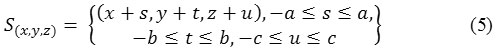
of size m* n, where m = 2a + 1 and n = 2b +1  are positive integers.

LEE Filter for Speckle

The Lee filter reduces the speckle noise by applying a spatial filter to each pixel in an image, which filters the data based on local statistics calculated within a square window. The value of the center pixel is replaced by a value calculated using the neighboring pixels [11]. This pointwise linear filter is based on the minimum mean square error (MMSE), and produced speckle noise free image based on the following equation (value of filtered pixel):

where,

and K= weight function,

—Center pixel value of kernel/window (Median value)

—Local mean of filter window

—Local variance of filter window

—Multiplicative noise mean (Default value: 1)

—Multiplicative noise variance (Default value: 0.25)

N Looks

Number of looks (Specifies the number of looks of the image. This is used to calculate the Multiplicative noise variance and control the amount of smoothing applied to the image. Using a smaller value for the Number of Looks leads to more smoothing, and a larger value preserves more image features [12].)

The N Looks for a homogeneous region of an image is the ratio between the mean squared to the variance. The N Looks is defined as follows:

The local mean L_m  of filter window is defined as (from eq. (5)):

Similarly, the local variance L_v of the filter window is defined as:

From eq. (8), if value of L_v is negative, in that case we have a very homogeneous area, L_v  should be set to zero. Then estimate

is given by the local mean L_m. If value of L_v is very high, this indicates a very high contrast region (or, an edge presence) and

These extreme cases are in accordance with the Bayesian approach that is adopted in this linear MMSE filter [1].

Frost Filter for Speckle

The FROST filter is used to design an adaptive filter algorithm to reduce speckle noise in spatial domain and computationally very efficient. This filter preserves the important features of image at the edges. It is a MMSE convolutional filter for speckle reduction. The Frost filter is an exponentially damped circularly symmetric filter that uses local statistics within individual filter windows. The pixel being filtered is replaced with a value calculated based on the distance from the filter center, the damping factor, and the local variance. The Frost filter requires a damping factor (define the extent of smoothing). The Damping Factor value defines the extent of exponential damping. The smaller the value is, the better the smoothing ability and filter performance. After application of the Frost filter, the denoised images show better sharpness at the edges [3], [7], [11], [13]. The algorithm used in the implementation of the Frost filter is as follows:

where,

and S—Absolute value of the pixel distance from the center pixel to its neighbors in the filter window,

D—Exponential damping factor (Default value:1)

The factor D is chosen such that when in a homogeneous region, B approaches zero, yielding the mean filter output; at an edge B becomes so large that filtering is inhibited completely [7].

Speckle Reducing Anisotropic Diffusion (SRAD) Filter

SRAD is a partial differential equation (PDE) technique for image enhancement and denoising. SRAD smooths the imagery and enhances edges by inhibiting diffusion across edges and allowing isotropic diffusion within homogeneous region [15].  Diffusion is a physical process to create equilibrium concentration differences without destroying or, creating body mass. This physical observation expressed equilibration property by Fick’s law of diffusion equation [4]:

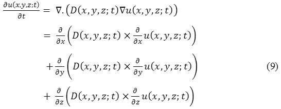
with initial condition u_o (x,y,z) = u (x, y, z; t = 0) which is noisy image/input image.

u (x, y, z; t) is the output image. D is diffusion coefficient, known as symmetric positive definite tensor, which depend on local structure of u (x, y, z; t)

(if D is constant, then filter is isotropic diffusion filter and if D is not constant, then filter is anisotropic diffusion filter) and ∇. and ∇ denote the divergence operator and gradient operator, respectively, u_o (x, y, z; t) is the initial image, i.e. noisy image, t is temporal variable. Eq. (9), Linear Anisotropic Diffusion (LAD), is an elliptic Partial Differential Equation (PDE). Here,

is a given field of symmetric positive definite diffusion tensors where Ω is an open region of ³ and ∂Ω  is boundary of Ω. Eigenvectors of these tensors define preferential diffusion directions, and the Eigenvalues their corresponding coefficients. Evolution rule eq. (9) is complemented with an initial condition u (x, y, z; 0) = u_o (x, y, z) at time t = 0. If u_o (x, y, z) has pixels of vector type, then their components are treated independently [6].

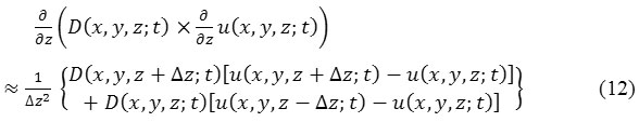
By using finite difference method, eq. (9) given as:

which is expressed as

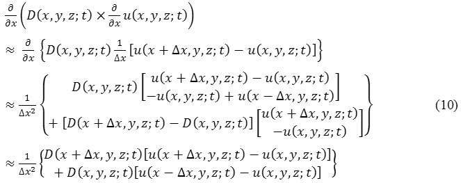
where “≈” shows that the R.H.S. part of the equation is the difference approximation of the L.H.S. part.

Similarly, we have

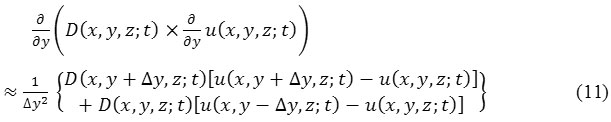
and

All the values of eq. (10), eq. (11), and eq. (12) inserting in eq. (9) to obtain difference approximation of

Put Δx = 1, Δy = 1, and Δz = 1 we get:

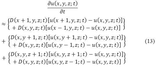
So, obtaining discrete realization of anisotropic diffusion filter for u (x, y, z; t) image from eq. (13):

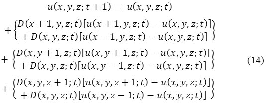
In eq. (14), we can see that the major problem is selection of diffusion coefficient D (x, y, z; t)  in anisotropic diffusion filter.

Most of the diffusion filters are simply modifications of perona-malik filter [5] where D is constant (scalar coefficient based on gradient of the image D∇ u (x, y, z; t) which avoids diffusion near the boundaries and applies it in homogeneous areas). To create a speckle imagery affected smooth region [7] propose a new anisotropic diffusion filter Speckle reducing anisotropic diffusion (SRAD). SRAD selects finite power intensity image u_o (x, y, z) and having none zero-valued intensities over the image domain Ω, and we get the output image u (x, y, z; t) by following PDE:

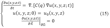
where ∂Ω  denotes the boundary of

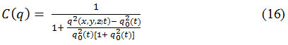
is the outer normal to the ∂Ω , and  C (q) is coefficient of diffusion which is defined as a decreasing function of the instantaneous coefficient of variation. Eq. (15) is known as SRAD PDE.

or,

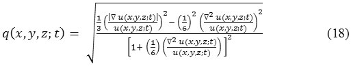
In eq. (16) and (17), q (x, y, z; t) is the instantaneous coefficient of variation serves as the edge detector in speckled imagery, q_o (t) is the speckle scale function and is estimation parameter related to the coefficient of variation of noise. q (x, y, z; t) is determined by:

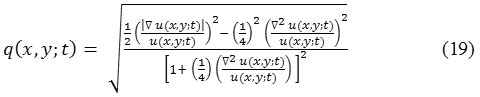
In case of 2-D, instantaneous coefficient of variation q (x, y; t):

Experimental Results

Images

We consider the two ‘true’ B-Mode US image of human kidney presented in [8] and [14] are used in this experiment, shown in figure 1. This real US image is used for quantitative analysis. The size of the both ‘true’ B-Mode US image of human kidney is 522x469x24 (figure 1(a)) and 640x445x24 (figure 1(b)) (in pixel unit) in x, y, and z directions respectively. For experiment purpose, we add speckle noise in both images with standard deviation σ = 0.4.

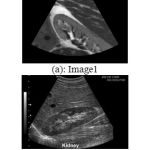Figure 1: Experiment results obtain from real B-mode US image of human kidney.   Click here to View figure

Performance Metrics

Two performance metrics were used in our experiments to measure the algorithm performance, one is called Peak Signal to Noise Ratio (PSNR) which is used for accuracy and precision of the ‘true’ image and other is called Structural Similarity Index Measure (SSIM) which is used for quality similarity between two images (original image and filtered image) [9].

Results

We select different parameter to compare the performance of four filters, named: Median filter, Lee Filter, Frost Filter, and SRAD filter. Initially, we fixed iteration number on 10, and vary window size as 3×3, 5×5, and 7×7. Then, fixed window size on 3×3 and vary iteration number as 20, 30, and 40. Table – 1 and Table – 2 in the Appendix – A shows performance of these different spatial filters in removing the speckle noise in image 1 and image 2 respectively, in terms of PSNR and SSIM performance index. The graphs show in figure 2 and figure 3 that SRAD filter is more efficient for removing Speckle noise in comparison to other stated filters, but the performance of median filter is also good enough for speckle noise reduction.

Table 1: PSNR and SSIM Results on Performance  comparison of  different filters for image 1

w=3, Iteration = 10			w=3, Iteration = 20
	PSNR	SSIM		PSNR	SSIM
LEE Filter	23.889	0.63966	LEE Filter	23.5837	0.61661
Frost Filter	23.8795	0.632	Frost Filter	23.5621	0.60863
SRAD Filter	25.7362	0.77948	SRAD Filter	43.7895	0.9745
Median Filter	24.3214	0.67509	Median Filter	23.7861	0.6123
w=5, Iteration = 10			w=3, Iteration = 30
	PSNR	SSIM		PSNR	SSIM
LEE Filter	23.4234	0.61548	LEE Filter	23.3994	0.60459
Frost Filter	23.3748	0.59612	Frost Filter	23.3757	0.5953
SRAD Filter	25.7437	0.79748	SRAD Filter	44.8842	0.9923
Median Filter	24.4718	0.6832	Median Filter	24.0041	0.6437
w=7, Iteration = 10			w=3, Iteration = 40
	PSNR	SSIM		PSNR	SSIM
LEE Filter	23.0825	0.60298	LEE Filter	23.2611	0.5955
Frost Filter	23.0267	0.57206	Frost Filter	23.2391	0.58599
SRAD Filter	25.8662	0.80847	SRAD Filter	45.0808	0.9966
Median Filter	25.1432	0.6995	Median Filter	24.2921	0.67221

Table 2: PSNR and SSIM Results on Performance comparison of  different filters for image 2

w=3, Iteration = 10			w=3, Iteration = 20
	PSNR	SSIM		PSNR	SSIM
LEE Filter	27.6073	0.71911	LEE Filter	26.1317	0.63893
Frost Filter	27.1898	0.70044	Frost Filter	25.9914	0.6208
SRAD Filter	30.4787	0.82994	SRAD Filter	29.5088	0.85245
Median Filter	29.7661	0.86084	Median Filter	26.0687	0.62511
w=5, Iteration = 10			w=3, Iteration = 30
	PSNR	SSIM		PSNR	SSIM
LEE Filter	25.7121	0.6231	LEE Filter	25.4983	0.60145
Frost Filter	25.4078	0.58327	Frost Filter	25.4248	0.58355
SRAD Filter	29.8732	0.8011	SRAD Filter	31.5179	0.95269
Median Filter	29.5625	0.8241	Median Filter	26.6608	0.65966
w=7, Iteration = 10			w=3, Iteration = 40
	PSNR	SSIM		PSNR	SSIM
LEE Filter	24.8834	0.58895	LEE Filter	25.1159	0.57862
Frost Filter	24.5747	0.53582	Frost Filter	25.0607	0.56113
SRAD Filter	29.2547	0.7961	SRAD Filter	34.5492	0.97378
Median Filter	29.1321	0.8019	Median Filter	27.7395	0.71693

 

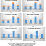Figure 2: The graphs are plotted for PSNR and SSIM result values for different filters (Image1). These graphs show that SRAD filter is more efficient for removing Speckle noise,but the performance of median filter is also good enough for Speckle noise reduction.   Click here to View figure

 

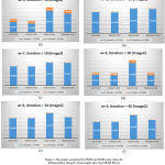Figure 3: The graphs are plotted for PSNR and SSIM result values for different filters (Image2). These graphs show that SRAD filter is more efficient for removing Speckle noise,but the performance of median filter is also good enough for Speckle noise reduction.   Click here to View figure

Conclusions

In this paper, we present a quantitative analysis of four filters: named: Median filter, Lee Filter, Frost Filter, and SRAD filter. These filters are used for speckle noise reduction. The performance analysis of these filters measure on the basis of the performance index PSNR and SSIM under different parameter selection. After the analysis with the help of corresponding result graphs, we conclude that SRAD filter is more efficient for removing Speckle noise in comparison to other stated filters, but the performance of median filter is also good enough for speckle noise reduction.

References

1. S. Lee, “Digital image enhancement and noise filtering by use of local statistics,” IEEE Trans. Pattern Anal. Mach. Intell., vol. PAMI-2, no. 2, pp. 165–168, Mar. 1980.
   CrossRef
2. Krissian, C.-F. Westin, R. Kikinis, and K. G. Vosburgh, “Oriented speckle reducing anisotropic diffusion,” IEEE Trans. Image Process., vol. 16, no. 5, pp. 1412–1424, May 2007.
   CrossRef
3. Frost, J. Stiles, K. Shanmugan, and J. Holzman, “A model for radar images and its application to adaptive digital filtering of multiplicative noise,” IEEE Trans. PAMI, vol. 4, no. 2, pp. 157–166, 1982.
   CrossRef
4. Weickert, Anisotropic Diffusion in Image Processing. Stuttgart, Germany: Teubner, 1998.
5. Perona and J. Malik, “Scale-space and edge detection using anisotropic diffusion,” IEEE Trans. Pattern Anal. Mach. Intell., vol. 12, no. 7, pp. 629–639, Jul. 1990.
   CrossRef
6. Jean-Marie Mirebeau, Jer^ome Fehrenbach, Laurent Risser, and Shaza Tobji,“Anisotropic Diffusion in ITK”, arXiv: 1503.00992v1 [cs.CV], March, 2015.
7. Yu and S. T. Acton, “Speckle reducing anisotropic diffusion,” IEEE Trans. Image Process., vol. 11, no. 11, pp. 1260–1270, Nov. 2002.
   CrossRef
8. Jorgen Arendt Jensen’s website, http://field-ii.dk/ for Field – II Simulation Program.
9. Sumit Kushwaha, “Mathematical Analysis of Robust Anisotropic Diffusion Filter for Ultrasound Images”, International Journal of Computer Sciences and Engineering, Volume-04, Issue-09, Page No (152-160), Sep -2016, E-ISSN: 2347-2693.
10. Arias-Castro and D.L. Donoho, “Does median filtering truly preserve edges better than linear filtering?”, Annals of Statistics, vol. 37, no. 3, pp. 1172 – 1206, 2009.
    CrossRef
11. ArcGIS for Desktop – Speckle Function, webpage available on: http://desktop.arcgis.com/en/arcmap/10.3/manage-data/raster-and-images/speckle-function.htm
12. Radar Enhanced Lee Filter, webpage available on: http://www.pcigeomatics.com/geomatica-help/concepts/orthoengine_c/chapter_825.html
13. Medical Image Processing – Techniques and Applications by Geoff Dougherty, Series: Biological and Medical Physics, Biomedical Engineering, Springer-Verlag New York , ISBN: 978-1-4614-3022-3, 2011.
14. Kidney Ultrasound Malaysia|Diagnostics Sonography for you, webpage available on: http://ultrasoundscanmalaysia.com/kidney-scan/
15. The Essential Guide to Image Processing by Alan C. Bovik, ELSEVIER, ISBN: 978-0-12-374457-9, 2009.
16. Wang, A. Bovik, H. Sheikh, and E. Simoncelli, “Image quality assessment: From error measurement to structural similarity,” IEEE Trans. Image Proces., vol. 13, no. 4, pp. 600–612, 2004.
    CrossRef
17. Elatrozy, A. Nicolaides, T. Tegos, A. Zarka, M. Griffin, and M. Sabetai, “The effect of B-mode ultrasonic image standardization of the echodensity of symptomatic and asymptomatic carotid bifurcation plaque,” Int. Angiology, vol. 17: 179–186, no. 3, 1998.
18. S. Lee, “Speckle analysis and smoothing of synthetic aperture radar images,” Computer Graph. & Image Proces., vol. 17, pp. 24–32, 1981.
    CrossRef
19. P. Loizou, C.S. Pattichis, C.I. Christodoulou, R.S.H. Istepanian, M. Pantziaris, and A. Nicolaides “Comparative evaluation of despeckle filtering in ultrasound imaging of the carotid artery,” IEEE Trans. Ultr. Ferroel. & Freq. Contr., vol. 52, no. 10, pp. 1653–1669, 2005.
    CrossRef
20. P. Loizou, C.S. Pattichis, M. Pantziaris, T. Tyllis, and A. Nicolaides, “Quantitative quality evaluation of ultrasound imaging in the carotid artery,” Med. Biol. Eng. Comput.,” vol. 44, no. 5, pp. 414–426, 2006.
    CrossRef
21. Greiner, C.P. Loizou, M. Pandit, J. Mauruschat, and F.W. Albert, “Speckle reduction in ultrasonic imaging for medical applications,” Proc. ICASSP91, Int. Conf. Acoustic Signal speech and Processing, Toronto Canada, May 14–17, pp. 2993-2996, 1991.
22. P. Loizou and C.S. Pattichis, “Despeckle filtering algorithms and Software for Ultrasound Imaging,” Synthesis Lectures on Algorithms and Software for Engineering, Morgan & Claypool Publishers, San Rafael, CA, 2008.

(Visited 1,556 times, 1 visits today)