
D. Selvathi1, N. B. Prakash2 , V. Gomathi3 and G. R. Hemalakshmi4
1Department of Electronics and Communication Engineering, Mepco Schlenk Engineering College, India.
2Department of Electrical and Electronics Engineering.
3,4Department of Computer Science and Engineering National Engineering College, India.
Corresponding Author E-mail: nbprakas@gmail.com
DOI : https://dx.doi.org/10.13005/bpj/1434
Abstract
Glaucoma frequently called as the "noiseless hoodlum of sight". The main source of visual impairment worldwide beside Diabetic Retinopathy is Glaucoma. It is discernible by augmented pressure inside the eyeball result in optic disc harm and moderate however beyond any doubt loss of vision. As the renaissance of the worsened optic nerve filaments isn't suitable medicinally, glaucoma regularly goes covered up in its patients anticipating later stages. All around it is assessed that roughly 60.5 million individuals beyond 40 years old experience glaucoma in 2010. This number potentially will lift to 80 million by 2020. Late innovation in medical imaging provides effective quantitative imaging alternatives for the identification and supervision of glaucoma. Glaucoma order can be competently done utilizing surface highlights. The wavelet channels utilized as a part of this paper are daubechies, symlet3 which will expand the precision and execution of classification of glaucomatous pictures. These channels are inspected by utilizing a standard 2-D Discrete Wavelet Transform (DWT) which is utilized to separate features and examine changes. The separated features are sustained into the feed forward neural system classifier that classifies the normal images and abnormal glaucomatous images.
Keywords
Anticipating; Augmented; Glaucomatous; Retinopathy
Download this article as:| Copy the following to cite this article: Selvathi D, Prakash N. B, Gomathi V, Hemalakshmi G. R. Fundus Image Classification Using Wavelet Based Features in Detection of Glaucoma. Biomed Pharmacol J 2018;11(2). |
| Copy the following to cite this URL: Selvathi D, Prakash N. B, Gomathi V, Hemalakshmi G. R. Fundus Image Classification Using Wavelet Based Features in Detection of Glaucoma. Biomed Pharmacol J 2018;11(2). Available from: http://biomedpharmajournal.org/?p=20606 |
Introduction
Glaucoma makes harm the eye’s optic nerve and deteriorates after a period of time as shown in Figure. 1. It’s frequently connected with a development of pressure inside the eye. The expanded pressure, called intraocular pressure can harm the optic nerve which passes on the pictures to our brain. On the off chance that harms to the optic nerve from high eye pressure proceeds with, glaucoma will cause perpetual loss of vision.
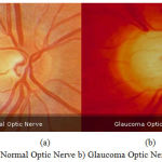 |
Figure 1a: Normal Optic Nerve b) Glaucoma Optic Nerve
|
Literature Survey
The most important step in the development process of the automation system is the documentation of comprehensive review of the published and unpublished work from secondary data sources in the areas of specific interest to the researcher. A review more often than not goes before the proposed framework and results segment. Its definitive objective is to convey the reader in the know regarding outgoing flow and structures the reason for another objective. A very much organized survey is described by an intelligent stream of thoughts, momentum and applicable references with predictable, suitable referencing style, appropriate utilization of wording, and a fair and extensive perspective of the past research on the theme.
Ganesh Babu et al present a new method for detection of glaucoma in the retinal images. The proposed system has three stages such as ROI Extraction, Feature Extraction and Classification. Digital image processing methods, for example, preprocessing, morphological tasks and thresholding, are generally utilized for the programmed recognition of optic disc, veins and estimation of the features. The features extracted are Cup to Disc Ratio (CDR) and the proportion of vessel area. K-means clustering method is utilized to compute the CDR feature and are validated by classifying the normal and glaucoma images using neural network classifier.
Acharya et al introduced glaucoma detection utilizing a mix of texture and higher order spectra (HOS) features. The results show that the texture and HOS includes after z-score standardization and feature determination, and when joined with a random forest classifier, performs superior to anything alternate classifiers and accurately distinguishes the glaucoma images with a decent exactness. The effect of feature positioning and standardization is additionally concentrated to enhance the outcomes. The features are clinically noteworthy and can be utilized to identify glaucoma precisely.
Huang.K et al done vitality circulation over wavelet sub groups is a generally utilized element for wavelet packet based texture arrangement. Because of the over total nature of the wavelet packet disintegration; include determination is typically connected for better grouping precision and minimal element portrayal. The larger part of wavelet feature choice calculations lead include choice in light of the assessment of each sub band independently, which verifiably accept that the wavelet features from various sub groups are autonomous. The reliance between features from various sub groups is researched hypothetically and mimicked for a given picture demonstrates. In view of analysis and simulation, a wavelet feature determination calculation in view of factual reliance is proposed. This algorithm is additionally enhanced by joining the reliance between wavelet include and the assessment of individual wavelet feature part. The results show the viability of the algorithms in fusing reliance into wavelet feature determination.
A.Arivazhagan et al defines the use of wavelet transform for classifying the texture of images by describing a new method of feature extraction for description and segmentation of texture at numerous scales based on block by block assessment of wavelet co-occurrence features. The steps involved in feature segmentation are decomposition of sub-image block, extraction, and successive block feature difference, and segmentation band, post processing and thinning. The execution of this algorithm is better than conventional single determination strategies, for example, texture spectrum, co-events and so on. The aftereffects of the proposed algorithm are observed to be acceptable. Efficiency is improved by removing noise using disk filtering and thresholding techniques.
Paul Y. Kim et al explores the utilization of fractal examination (FA) as the premise of a framework for multiclass forecast of the movement of glaucoma. FA is connected to pseudo 2-D pictures changed over from 1-D retinal nerve fiber layer information acquired from the eyes of ordinary subjects, and from subjects with dynamic and non dynamic glaucoma. FA features are acquired utilizing a box-counting technique and a multifractional Brownian movement strategy that consolidates texture and multiresolution examinations. The two features are utilized for Gaussian kernel based multiclass classification. Sensitivity, specificity, and area under receiver operating characteristic (AUROC) are computed for the FA features and for measurements got utilizing Wavelet-Fourier analysis (WFA) and Fast-Fourier analysis (FFA). Synchronous multiclass characterization among progressors, nonprogressors, and visual typical subjects has not been already portrayed. The novel FA-based features accomplish better execution with less features and less computational than WFA and FFA.
Jun Cheng et al proposes optic disc and optic cup segmentation using super pixel classification for glaucoma screening. In optic disc segmentation, histograms, and center surround statistics are used to classify each super pixel as disc or non-disc. For optic cup division, notwithstanding the histograms and focus encompass measurements, the area data is likewise included into the component space to help the execution. The proposed segmentation strategies have been assessed in a database of 650 images with OD and OC limits physically set apart via trained experts. The segmented OD and OC are then used to process the CDR for glaucoma screening. The technique accomplishes AUC of 0.800 and 0.822 in two different databases, which is higher than other strategies. The techniques can be utilized for glaucoma screening. The effective quantitative imaging alternatives for the detection and management of glaucoma. Several imaging modalities and their enhancements, including optical coherence tomography and multifocal electro retinograph are prominent techniques employed to quantitatively analyze structural and functional abnormalities in the eye both to observe variability and to quantify the progression of the disease objectively. Automated clinical decision support systems (CDSSs) in ophthalmology, such as CASNET/glaucoma are designed to create effective decision support systems for the identification of disease pathology in human eyes.
Texture assumes a critical part in numerous machine vision errands, for example, surface examination, scene classification, surface introduction and shape assurance. Texture is portrayed by the spatial dissemination of gray levels in an area. Analysis of texture requires the identification of proper attributes or features that differentiate the textures in the image for segmentation, classification and recognition. The features are assumed to be uniform within the regions containing the same textures. Textural features are, consequently, not bound to particular areas on the image. A few component extraction systems, including spectral procedures, are accessible to mine texture features. The utilization of texture features and HOS were proposed for glaucomatous classification. In spite of the fact that the texture based strategies have been demonstrated effective, it is as yet a test to produce includes that recover summed up auxiliary and textural features from retinal images. Textural features utilizing Wavelet Transforms (WTs) in image processing are frequently utilized to conquer the generalization of features.
Datasets
This database was recognized by a study group to carry proportional studies on automatic segmentation algorithms on fundus images. The public dataset examples shown in Figure.2 consist of 15 healthy fundus, 15 DR images and 15 glaucomatous images. Binary gold standard vessel segmentation images are available and also masks influential FOV are provided.
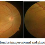 |
Figure 2: Typical fundus images-normal and glaucoma
|
Proposed System
The objective of this work is to differentiate normal eye images and glaucoma affected eye images. This classification is based on selecting eminent features using wavelet filters. The wavelet features are used to train the supervised classifier which classifies retinal images into normal or abnormal and achieve a high a level of accuracy as shown in Figure.3. It is proposed to use a wavelet filter is daubechies. This filter is used to calculate energy and average value for the image. With the help of this filter, the wavelet coefficients are obtained and their characteristics like average, energy, standard deviation and variance are resulting in feature extraction. This filter will increase the accuracy and performance of an image. This filter is examined by employing a standard 2-D discrete wavelet transform (DWT) which are used to extract features and analyze changes. The extracted features are fed into supervised classifier such as Neural Network.
The figure 6.1 describes about the overall process architecture of our project. There will be sets like training set and testing set. In training set the input images that are to be trained are preprocessed. The preprocessing is carried out like scaling and selecting green channel. Then from the preprocessed input images, features like average, energy, standard deviation and variance are extracted. Then these extracted features are fed into Neural Network classifier for classification process. In testing set, each image that is tested whether it is normal or abnormal.
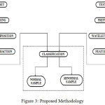 |
Figure 3: Proposed Methodology
|
Preprocessing
The objective of preprocessing is to improve the interoperability of the information present in images for human viewers. An enhancement algorithm is one that yields a better quality image for the purpose of some particular application which can be done by either suppressing the noise or increasing the image contrast. Image preprocessing includes emphasis, sharpen or smoothen image features for display and analysis. Enhancement methods are application specific and are often developed empirically. Image preprocessing techniques emphasis specific image features to improve the visual perception of an image.
Image Decompositon using Wavelet Transforms
The DWT confine the spatial and frequency information’s of an indication. DWT breaks down the image by disintegrating it into a coarse estimate through low-pass filtering and into detail data by means of high-pass filtering. Such decay is performed recursively on low-pass estimate coefficients got at each level, until the point when the vital emphases are come to. Each image is represented to as a p × q gray scale network I [i,j], where every component of the framework speaks to the grayscale intensity of one pixel of the image. Each nonborder pixel has eight nearby neighboring pixel intensities. These eight neighbors can be utilized to navigate the network. The resultant 2-D DWT coefficients are the same regardless of whether the lattice is crossed ideal left-to-right or right-to-left. Henceforth, it is adequate that we consider four directions comparing to 0◦ (Dh), 45◦ (Dd), 90◦ (Dv), and 135◦ (Dd) orientations. The decay structure for one level is represented in Figure.4. In this work daubechies (db4) wavelet filter is used. After decomposition, it reproduces the original image without loss of any information. The proposed system contains features of average or mean, energy, standard deviation and variance.
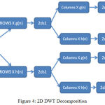 |
Figure 4: 2D DWT Decomposition
|
Feature Extraction
It is used to select important features of an image. Feature extraction is a particular form of dimensionality reduction. If the input data is too large to be processed, then the input information will be transformed into a condensed set of features (also named features vector). The features extracted are carefully chosen such a way that they will extract the relevant information to carry out the desired task. This approach is successful when images are large and an optimized features is required to complete tasks quickly.
Investigation with an extensive number of factors by and large requires a lot of memory and computation control or classification method which over fits the training sample and sums up inadequately to new examples. Best outcomes are accomplished when a specialist develops an arrangement of use of application dependent features.
Average or Mean
Average feature helps to measure the center tendency of data. Average is Add up all the numbers (pixels) and then divided by the number of pixels. It is calculated from the decomposition image in directions of horizontal, vertical and diagonal as stated in Equation (1 to 3).
Energy
It is the proportion of each channel takes up in original color image or which channel (Red, Green and Blue) has the bigger proportion and has been calculated as stated in Equation (4 to 6)
Standard Deviation
The standard deviation (SD) as stated in Equation (7) describes the variation from the average exists. A low SD point towards that the data points are close to the mean. A high SD point towards that the data points are extensive over huge values.
Variance
The difference measures how far an arrangement of numbers is spread out. (A difference of zero demonstrates that every one of the qualities are indistinguishable.) Variance is dependably non-negative. A little fluctuation demonstrates that the information directs incline toward be near the mean (expected esteem) and henceforth to each other, while a high change shows that the information calls attention to extremely spread out from the mean and from each other. The square foundation of change is known as the standard deviation. Square of standard deviation gives an estimate spread of pixel value around the image mean.
Image Classification
Classification of data is used to assign corresponding levels with the aim of discriminating multiple objects from each other within the image. The level is called as class. Classification will be executed on the base of spectral or spectrally defined features, such as density, texture etc. It can be said that classification divides the feature space into several classes based on a decision rule. In this work, the classification process has been carried out as per the flow diagram shown in Figure. 5.
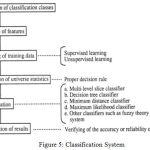 |
Figure 5: Classification System
|
Neural systems are made out of basic components working in parallel. These components are motivated by natural sensory systems. As in nature, the associations between components generally decide the system work. Neural system can be prepared to play out a specific capacity by changing the estimations of the associations (weights) between components. Commonly, neural systems are balanced, or prepared, with the goal that a specific info prompts a particular target yield. The system is balanced, in light of a correlation of the yield and the objective, until the point when the system yield coordinates the objective. Regularly, numerous such info/target sets are expected to train the system.
Results and Discussion
The feature information extracted for healthy and glaucomatous input image along horizontal, vertical and diagonal axis is tabulated in Table 1 to Table 6. The values are calculated for average for red, green and blue channels. Energy, standard deviation and variance are calculated for green channel.
Table 1: Glaucoma image-horizontal detail
| Image | Average | Energy | Standard Deviation | Variance | ||
| Red | Green | Blue | ||||
| 1_g | 0.4812 | 0.8771 | 1.0113 | 7.5687e-007 | 18.9651 | 1.0240e+007 |
| 2_g | 0.4318 | 0.5440 | 0.6198 | 1.3168e-010 | 0.2510 | 0.2849 |
| 3_g | 0.3098 | 0.5161 | 0.5870 | 1.0832e-010 | 0.2023 | 0.1428 |
| 4_g | 0.4033 | 0.5475 | 0.6367 | 1.1462e-010 | 0.1848 | 0.1120 |
| 5_g | 0.4646 | 0.5552 | 0.6490 | 1.3220e-010 | 0.2374 | 0.2365 |
| 6_g | 0.4860 | 0.4590 | 0.5319 | 7.2313e-011 | 0.1713 | 0.0675 |
| 7_g | 0.2435 | 0.5227 | 0.6208 | 1.8193e-010 | 0.4990 | 3.4628 |
| 8_g | 0.3384 | 0.4717 | 0.5618 | 8.5429e-011 | 0.2072 | 0.1393 |
| 9_g | 0.4299 | 0.5456 | 0.6596 | 1.6108e-010 | 0.3100 | 0.5052 |
| 10_g | 0.5223 | 0.4949 | 0.5719 | 9.8881e-011 | 0.2313 | 0.1655 |
| 11_g | 0.5302 | 0.4909 | 0.5817 | 9.0322e-011 | 0.1785 | 0.0817 |
| 12_g | 0.5231 | 0.5116 | 0.5937 | 1.2108e-010 | 0.2562 | 0.5398 |
| 13_g | 0.4512 | 0.6618 | 0.7664 | 2.1839e-007 | 6.0759 | 2.4196e+005 |
| 14_g | 0.4432 | 0.4504 | 0.5261 | 6.0745e-011 | 0.1477 | 0.0395 |
| 15_g | 0.4992 | 0.4715 | 0.5540 | 7.7145e-011 | 0.1974 | 0.1634 |
Table 2: Healthy image-horizontal detail
| Image | Average | Energy | Standard Deviation | Variance | ||
| Red | Green | Blue | ||||
| 1_h | 0.6136 | 0.6112 | 0.7181 | 1.6934e-010 | 0.1974 | 0.1681 |
| 2_h | 0.6679 | 0.7609 | 0.8839 | 1.8858e-007 | 4.2578 | 9.3808e+004 |
| 3_h | 0.6645 | 0.6209 | 0.7246 | 1.8141e-010 | 0.2396 | 0.3420 |
| 4_h | 0.6734 | 0.8035 | 0.9290 | 4.0788e-007 | 6.2043 | 4.0729e+005 |
| 5_h | 0.6251 | 0.6057 | 0.7140 | 1.6570e-010 | 0.2160 | 0.2110 |
| 6_h | 0.5842 | 0.5475 | 0.6378 | 1.1106e-010 | 0.1723 | 0.0885 |
| 7_h | 0.4696 | 0.5197 | 0.6171 | 9.1439e-011 | 0.1533 | 0.0569 |
| 8_h | 0.5297 | 0.5186 | 0.6055 | 9.1857e-011 | 0.1590 | 0.0594 |
| 9_h | 0.5945 | 0.6513 | 0.7768 | 1.0330e-007 | 3.7624 | 4.7189e+004 |
| 10_h | 0.2628 | 0.4721 | 0.5608 | 8.1885e-011 | 0.2025 | 0.1241 |
| 11_h | 0.4195 | 0.4770 | 0.5638 | 8.9989e-011 | 0.2338 | 0.2123 |
| 12_h | 0.4485 | 0.4382 | 0.5278 | 5.7557e-011 | 0.1412 | 0.0317 |
| 13_h | 0.4208 | 0.4196 | 0.4983 | 4.7774e-011 | 0.1477 | 0.0406 |
| 14_h | 0.5008 | 0.4477 | 0.5305 | 5.9895e-011 | 0.1514 | 0.0437 |
| 15_h | 0.4271 | 0.4704 | 0.5668 | 7.6932e-011 | 0.1726 | 0.0710 |
Table 3: Healthy image vertical detail
| Image | Average | Energy | Standard Deviation | Variance | ||
| Red | Green | Blue | ||||
| 1_h | 0.4508 | 0.4456 | 0.5132 | 5.3351e-011 | 0.2550 | 0.1157 |
| 2_h | 0.5461 | 0.5050 | 0.5731 | 9.1708e-011 | 0.3231 | 0.4364 |
| 3_h | 0.4949 | 0.4594 | 0.5318 | 5.9957e-011 | 0.2590 | 0.1239 |
| 4_h | 0.5882 | 0.7387 | 0.8566 | 5.4588e-007 | 5.3246 | 1.4883e+005 |
| 5_h | 0.4624 | 0.4403 | 0.5049 | 4.9679e-011 | 0.2424 | 0.0851 |
| 6_h | 0.4870 | 0.4583 | 0.5223 | 5.8817e-011 | 0.2603 | 0.1235 |
| 7_h | 0.4648 | 0.5063 | 0.5808 | 8.8520e-011 | 0.3057 | 0.2697 |
| 8_h | 0.5113 | 0.4977 | 0.5674 | 7.9265e-011 | 0.2814 | 0.2113 |
| 9_h | 0.5818 | 0.7459 | 0.9042 | 1.4748e-006 | 9.7181 | 1.4898e+006 |
| 10_h | 0.2536 | 0.4556 | 0.5393 | 6.5747e-011 | 0.3123 | 0.3574 |
| 11_h | 0.3747 | 0.4115 | 0.4852 | 4.5316e-011 | 0.2891 | 0.3297 |
| 12_h | 0.4369 | 0.4296 | 0.5009 | 5.2482e-011 | 0.2868 | 0.2666 |
| 13_h | 0.4613 | 0.4480 | 0.5412 | 6.2309e-011 | 0.3178 | 0.3830 |
| 14_h | 0.4756 | 0.4285 | 0.5024 | 5.0414e-011 | 0.2839 | 0.2654 |
| 15_h | 0.4141 | 0.4519 | 0.5419 | 6.8852e-011 | 0.3400 | 0.4976 |
Table 4: Glaucoma image vertical detail
| Image | Average | Energy | Standard Deviation | Variance | ||
| Red | Green | Blue | ||||
| 1_g | 0.4310 | 0.7237 | 0.8336 | 1.4816e-007 | 4.8549 | 1.2669e+005 |
| 2_g | 0.4547 | 0.5645 | 0.6166 | 2.3765e-010 | 0.8150 | 26.5541 |
| 3_g | 0.3236 | 0.5283 | 0.5964 | 1.1447e-010 | 0.3785 | 0.8233 |
| 4_g | 0.3800 | 0.5128 | 0.5779 | 9.6839e-011 | 0.3348 | 0.4559 |
| 5_g | 0.4006 | 0.4552 | 0.5327 | 5.5548e-011 | 0.2474 | 0.1009 |
| 6_g | 0.4794 | 0.4379 | 0.5222 | 5.6051e-011 | 0.2986 | 0.2805 |
| 7_g | 0.2419 | 0.4571 | 0.5443 | 6.7806e-011 | 0.3190 | 0.3853 |
| 8_g | 0.3160 | 0.4332 | 0.5015 | 5.3473e-011 | 0.2918 | 0.2658 |
| 9_g | 0.3541 | 0.4269 | 0.5254 | 5.4800e-011 | 0.3119 | 0.3446 |
| 10_g | 0.4515 | 0.4240 | 0.4935 | 5.1685e-011 | 0.3048 | 0.3002 |
| 11_g | 0.5895 | 0.6696 | 0.7858 | 2.9179e-007 | 3.7750 | 4.1048e+004 |
| 12_g | 0.4796 | 0.4622 | 0.5407 | 7.1540e-011 | 0.3472 | 0.5457 |
| 13_g | 0.3978 | 0.4367 | 0.5249 | 5.7391e-011 | 0.3062 | 0.3196 |
| 14_g | 0.4131 | 0.4226 | 0.4814 | 4.8108e-011 | 0.2704 | 0.1902 |
| 15_g | 0.4283 | 0.4066 | 0.4674 | 4.5561e-011 | 0.2937 | 0.2401 |
Table 5: Healthy image diagonal detail
| Image | Average | Energy | Standard Deviation | Variance | ||
| Red | Green | Blue | ||||
| 1_h | 0.2285 | 0.2344 | 0.2560 | 3.8383e-012 | 0.0454 | 2.6882e-004 |
| 2_h | 0.2542 | 0.2429 | 0.2617 | 4.4430e-012 | 0.0492 | 3.6265e-004 |
| 3_h | 0.2590 | 0.2477 | 0.2705 | 4.8065e-012 | 0.0537 | 4.7968e-004 |
| 4_h | 0.2390 | 0.2293 | 0.2467 | 3.5597e-012 | 0.0423 | 2.3726e-004 |
| 5_h | 0.2358 | 0.2330 | 0.2541 | 3.7117e-012 | 0.0438 | 2.5080e-004 |
| 6_h | 0.2342 | 0.2223 | 0.2418 | 3.2085e-012 | 0.0399 | 1.6688e-004 |
| 7_h | 0.2042 | 0.2312 | 0.2532 | 3.8611e-012 | 0.0493 | 4.2539e-004 |
| 8_h | 0.2263 | 0.2294 | 0.2469 | 3.5275e-012 | 0.0413 | 2.1406e-004 |
| 9_h | 0.2024 | 0.1940 | 0.2086 | 2.0859e-012 | 0.0323 | 7.7290e-005 |
| 10_h | 0.1139 | 0.2137 | 0.2316 | 2.8535e-012 | 0.0367 | 1.6540e-004 |
| 11_h | 0.1734 | 0.2032 | 0.2184 | 2.4664e-012 | 0.0335 | 9.8718e-005 |
| 12_h | 0.1999 | 0.2044 | 0.2209 | 2.6008e-012 | 0.0349 | 1.1299e-004 |
| 13_h | 0.1889 | 0.1944 | 0.2124 | 2.0995e-012 | 0.0311 | 7.7913e-005 |
| 14_h | 0.2123 | 0.2018 | 0.2144 | 2.3296e-012 | 0.0288 | 5.6364e-005 |
| 15_h | 0.1932 | 0.2201 | 0.2435 | 3.1807e-012 | 0.0381 | 1.7156e-004 |
Table 6: Glaucoma image diagonal detail
| Image | Average | Energy | Standard Deviation | Variance | ||
| Red | Green | Blue | ||||
| 1_G | 0.1548 | 0.2353 | 0.2536 | 4.7799e-012 | 0.0670 | 0.0011 |
| 2_G | 0.1877 | 0.2347 | 0.2488 | 3.9901e-012 | 0.0485 | 3.0642e-004 |
| 3_G | 0.1321 | 0.2236 | 0.2414 | 3.1381e-012 | 0.0389 | 1.5426e-004 |
| 4_G | 0.1723 | 0.2372 | 0.2569 | 4.0093e-012 | 0.0432 | 2.3126e-004 |
| 5_G | 0.1849 | 0.2214 | 0.2420 | 3.2582e-012 | 0.0434 | 2.5581e-004 |
| 6_G | 0.2081 | 0.1983 | 0.2139 | 2.2808e-012 | 0.0355 | 1.4045e-004 |
| 7_G | 0.1090 | 0.2261 | 0.2455 | 3.5995e-012 | 0.0452 | 3.2754e-004 |
| 8_G | 0.1439 | 0.2070 | 0.2237 | 2.6756e-012 | 0.0373 | 1.7287e-004 |
| 9_G | 0.1720 | 0.2211 | 0.2431 | 3.2330e-012 | 0.0400 | 1.8912e-004 |
| 10_G | 0.2146 | 0.2113 | 0.2245 | 2.7072e-012 | 0.0368 | 1.3646e-004 |
| 11_G | 0.2162 | 0.2089 | 0.2302 | 2.7315e-012 | 0.0346 | 1.0772e-004 |
| 12_G | 0.2182 | 0.2205 | 0.2363 | 3.2593e-012 | 0.0406 | 2.0156e-004 |
| 13_G | 0.1717 | 0.1995 | 0.2170 | 2.4236e-012 | 0.0310 | 7.1496e-005 |
| 14_G | 0.1770 | 0.1855 | 0.1991 | 1.9719e-012 | 0.0348 | 6.5016e-005 |
| 15_G | 0.1998 | 0.1994 | 0.2112 | 2.3862e-012 | 0.0392 | 1.3793e-004 |
The features along horizontal, vertical and diagonal axis of the image extracted are fetched as input to FFBNN classifier in order to train and test the system. The neural network performance platform and the classification output for both healthy and abnormal image is shown in Figure.6 to Figure.9.
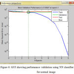 |
Figure 6: GUI showing performance validation using NN classifier for normal image
|
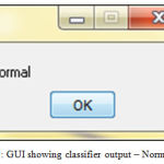 |
Figure 7: GUI showing classifier output – Norma
|
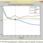 |
Figure 8: GUI showing performance validation using NN classifier for abnormal image
|
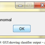 |
Figure 9: GUI showing classifier output – Abormal
|
Table 7 gives the results of the proposed work on HRF dataset shows the performance evaluation of classification of fundus image, and an average sensitivity rate of 100% and specificity rate of 91.67% and accuracy rate of 95.83% on HRF dataset are obtained.
Table 7: Performance measurement
| Classes | No. of Training Images | No. of Testing Images | No. of Correctly Classified Images | Classification Accuracy (%) |
| Normal | 05 | 12 | 12 | 100 |
| Glaucoma | 05 | 12 | 11 | 91.67 |
| Average Accuracy | 95.83 | |||
Table 8 shows the performance comparisons of the proposed classification methodology with the authors Kiran S.M et al (2016) and N.Annu et al (2013). The proposed methodology achieves 95.83% average accuracy compared with the Kiran S.M et al (2016) achieves 91.66% of an average accuracy and N.Annu et al (2013) achieves 95% of an average accuracy. This proposed classification methodology on HRF dataset provides better sensitivity and higher accuracy.
Table 8: Performance comparison of Glaucoma classification
| Methodologies | Year | Accuracy (%) |
| Proposed work | 2017 | 95.83 |
| Kiran SM et al [13] | 2016 | 91.66 |
| N.Annu et al [14] | 2013 | 95.00 |
Conclusion
The proposed method to classify the fundus image into normal and glaucomatous image is carried out in this work. The results obtained yield an accuracy rate of 95.83%. The study also illustrates the efficacy of wavelet-based feature techniques for detecting and predicting glaucomatous progression. From the accuracies obtained, it can be concluded that the average, energy, standard deviation and variance are obtained from the detailed coefficients that can be used to distinguish between normal and glaucomatous images with very high level accuracy.
Conflict of Interest
The authors declare that there is no conflict of interest with respect to the above research work.
References
- Sisodia D.S, Nair S, Khobragade P. Diabetic Retinal Fundus Images: Preprocessing and Feature Extraction for Early Detection of Diabetic Retinopathy. Biomed Pharmacol J. 2017; 10(2): 615-626.
CrossRef - Kiran SM and Chandrappa DN. Automatic Detection of Glaucoma using 2-D DWT. International Research Journal of Engineering and Technology. 2016; 3(6): 201-205.
- Ganesh Babu, TR, Sathishkumar, R & Rengarajvenkatesh. Segmentation of optic nerve head for glaucoma detection using fundus images. Biomedical and Pharmacology Journal. 2014; 7(2): 697-705.
CrossRef - Annu N and Judith Justin. Automated Classification of Glaucoma Images by Wavelet Energy Features. International Journal of Engineering and Technology, 2013; 5(2): 1716-1721.
- Paul Y. Kim, Khan M. Iftekharuddin, Pinakin G. Davey, Márta Tóth, Anita Garas, Gabor Holló, Edward A. Essock. Novel Fractal Feature-Based Multiclass Glaucoma Detection and Progression Prediction. IEEE Journal of Biomedical and Health Informatics. 2013; 17(2) 269–276.
CrossRef - Jun Cheng, Jiang Liu, Yanwu Xu, Fengshou Yin, Damon Wing Kee Wong, Ngan-Meng Tan, Dacheng Tao, Ching-Yu Cheng, Tin Aung, Tien Yin Wong. Superpixel Classification Based Optic Disc and Optic Cup Segmentation for Glaucoma Screening. IEEE Transactions on Medical Imaging, 2013; 32(6): 1019–1032.
CrossRef - Dua, Sumeet U. Rajendra Acharya, Pradeep Chowriappa, and S. Vinitha Sree. Wavelet-Based Energy Features for Glaucomatous Image Classification. IEEE Transactions on Information Technology in Biomedicine. 2012.
- U. Rajendra Acharya, Sumeet Dua, Xian Du, Vinitha Sree S, Chua Kuang Chua. Automated Diagnosis of Glaucoma Using Texture and Higher Order Spectra Features. IEEE Transactions on Information Technology in Biomedicine. 2011; 15(3): 449–455.
CrossRef - Balasubramanian et al., Clinical evaluation of the proper orthogonal decomposition framework for detecting glaucomatous changes in human subjects. Invest Ophthalmol Vis Sci. 2010; 51(1): 264–271.
CrossRef - J.M. Miquel-Jimenez et al., Glaucoma detection by wavelet-based analysis of the global flash multifocal electroretinogram. Eng. Phys. 2010; 32: 617–622.
CrossRef - Ke Huang, Selin Aviyente. Wavelet Feature Selection for Image Classification. IEEE Transactions on Image Processing. 2008; 17 (9): 1709 – 1720
CrossRef - Arivazhagan, L. Ganesan. Texture segmentation using wavelet transform’ Pattern Recognition Letters, 2003; 24: 3197-3203.
CrossRef

