Sanjay H. S¹, Bhargavi S² and Dinesh P. A.³  

¹Research Scholar, Jain University and Assistant Professor, Dept of Medical Electronics, MSRIT, Bangalore.

²Departmen of Telecommunication Engg, SJC Institute of Technology, Chikkaballapura.

³Department of Mathematics, MSRIT, Bangalore.

Corresponding Author E-mail: sanjaymurthyhs@gmail.com

DOI : https://dx.doi.org/10.13005/bpj/1252

Abstract

Psychophysics and temporal resolution and often linked to each other. The ability of an individual to resolve a given sensory input temporally is the cue for a better perception of the same. While sensation could be from visual, tactile, olfactory or somatosensory, the present paper emphasizes on the assessment of the psychophysics of the temporal resolution of a given auditory input and hence the perception based analysis of the given set of individuals. 44 subjects of no known auditory pathological history have been considered for this study. Two categories of subjects namely employees of chemical industries and professional basketball players are considered for this experiment. The subjects are made to undergo two tests, Frequency Response Test (FRT) and Absolute Threshold Test (ATT). The results show a clear distinction between the two groups of study proving the variations in the auditory perception due to their exposure to solvents in chemical industries and because of the regular playing of basketball game on a professional front proving the effects of desired conditioning due to regular training in sports such as basketball and undesired conditioning due to occupation exposure to noise and solvents with respect to the psychophysical variations of auditory temporal resolution in human beings

Keywords

Auditory Temporal Resolution; Absolute Threshold; occupational exposure Frequency Response; Psychophysics;

Download this article as: 

Copy the following to cite this article: Sanjay H. S, Bhargavi S, Dinesh P. A. Auditory Temporal Resolution Based Psychophysical Evaluation of Healthy Individuals Exposed to Desired and Undesired Conditioning. Biomed Pharmacol J 2017;10(3).

Copy the following to cite this URL: Sanjay H. S, Bhargavi S, Dinesh P. A. Auditory Temporal Resolution Based Psychophysical Evaluation of Healthy Individuals Exposed to Desired and Undesired Conditioning. Biomed Pharmacol J 2017;10(3). Available from: http://biomedpharmajournal.org/?p=16570

Introduction

Frequency and intensity are the most important attributes of sound and hence can aid in the assessment of variations in the perception of sound by human beings.¹ Conventional diagnostics tests such as audiometry often fail to assess the variations in non-pathological cases and hence there is a need to develop alternate approaches with respect to hearing perception based variations in normal human beings which can be due to their regular routine or occupation.² One such case is the chemical industries where exposure to solvents is known to be a definite cause towards the deterioration of hearing. This aspect is often neglected in developing countries such as India where more emphasis is not provided towards preventive diagnostics or early detection.³ Hence it is of prime importance to assess the pattern and plausible degradation of hearing with the aid of the variation in the hearing perception which is a cue towards the initiation of the deterioration of the auditory functions.⁴ With regard to the same, sports such as basketball and table tennis requires a higher level of auditory temporal resolution in order to perform better and hence such players would have naturally improved on their auditory temporal resolution based aspects due to regular training in these sports.⁵ Hence it is apt to conclude that basketball players have a better abilities with respect to hearing perception as compared to the employees of chemical industries who’s perception would be affected in an adverse manner due to their occupational exposure.⁶ Although the hearing abilities may seem to be normal in both these cases, it is necessary to assess the same with the aid of FRT and ATT in order to obtain a better conclusion about the hearing perception based abilities in such individual⁷

Background

Frequency Response

Frequency response in general terms is the output spectrum of a system when subjected to a set of stimuli which helps understand the dynamics of the system. Hence in terms of hearing, frequency response is the output spectrum of the system ear for a set of stimuli which is the varying levels of intensity given over a range of frequencies. When we want to determine how well something is able to “hear”, our best option is to use the frequency response concept. To understand that as quantifiable results, the response of the system is evaluated over a range of frequencies. The system can be anything from microphones or loudspeakers to the human ear. The human hearing ranges roughly from 20 Hz to 20000 Hz. The most sensitive range of the human ear is approximately at 3500 to 4000 Hz. This means that a normal human being can detect the lowest sounds of even 0 dB SPL at 3KHz but can merely detect a 40 dB SPL sound at 100 Hz.⁸

Threshold Estimation

Estimation of hearing threshold is generally performed using discrimination based approach of detection based approach. In discrimination based approach, the task is to differentiate between given two sounds. In detection based approach, the task would be to detect the presence of sound and not differentiate between multiple sounds. This can be a simple yes/no answer while the discrimination based tests are more complex. Detection based tests can be designed based on adaptive / non-adaptive protocols where the attributes of sound are varied based on the previous responses of the subject in case of adaptive methods and conventionally follow a certain pre-defined patterns such as ramp, staircase etc in case of  non-adaptive approach without considering the response of the subject⁹

Absolute Threshold

Absolute thresholds are measured using maximum likelihood approach. Pure tone of 1 KHz and 500 msec are presented to the subject. The tone is designed using various approaches. The subject is asked to respond if they tome was heard or not and based on this response, the threshold value of the hearing perception is calculated. Many more approaches such as staircase, neural network based approaches exist to design absolute threshold assessment paradigm. ¹⁰

Chemical Industries

There are industrial chemicals that are ototoxic (poisonous to the ears), meaning that they can damage hearing just as easily as industrial noise. However, simultaneous exposure to noise and ototoxic chemicals is particularly insidious because of their synergistic effect. This causes damage to the inner ear and the auditory neurological pathway which further leads to loss of hearing. Damage to hearing is more likely if there is an exposure to noise with chemicals or even with a combination of more than one chemical. Ototoxic chemicals are divided into workplace chemicals and medication. Only a few of the Ototoxic chemicals have been studied in depth but more than 750 are considered to be potentially ototoxic. Cochleotoxic chemical such as aspirin and non-steroidal anti-inflammatory drugs too affect the hearing functions. Such medications, with a noise exposure can cause sensorineural hearing disorders. Although much work is being done with such approaches, very little research is in progress towards industrial exposure to noise and chemicals in daily life which is the need of the hour.¹¹

Basketball Players

It is a known fact that sports help in the overall development of an individual and is a definite reason in the betterment of various physical and physiological aspects as well. In this context, certain games such as table tennis, basketball and cricket help in the improvisation of the overall temporal resolution in the individuals. In other words, a professional basketball player is known to have a better hearing perception than a non-player. One could also say that for an individual to play better, it is very important to have a better perception based abilities. Else the overall performance would reduce and hence this is a very important aspect of training as well as in case of sports rehabilitation.¹²

Methodology

Subjects

44 subjects of age group 20-50 years with no known auditory pathological history or any kind of hearing dysfunction were chosen for this experiment. Two sets, one being the employees of chemical industries with an experience of atleast 3 years in the domain with definite exposure to solvents in their occupation, regarded to be undesired conditioning was considered to be the chemical industry subjects. The other group included professional basketball players who were known to be playing basketball for a minimum of 3 years and were selected into their respective college teams during this period and concluded to be desired conditioning subjects. These players were known to be involved with a regular routine of basketball practice during these 3 years. The FRT was conducted during the morning slot (8.00 am – 10.00 am) for the subjects. For the chemical industry subjects, this was considered to be the time before their entry into their work place in order to begin their shifts. In case of basketball players, this was the slot before their regular morning practice commenced The ATT was conducted once in the morning (8.00 am – 10.00 am) and also in the evening ( 4.00 pm – 6.00 pm) after their work shift in case of chemical industry employees and after their regular evening practice slot in case of basketball players. Both FRT and ATT were conducted in a noise free environment with the aid of a sony vio laptop and Panasonic HD headphones. MATLAB tool was used for the generation and presentation of the sounds with variations in frequency and intensity during tests. For the FRT, the hearing test tool was used and for ATT, Psychoacoustics toolbox was used for data acquisition in MATLAB^13,14

Frequency Response Test (FRT)

Frequency Response (FR) is often considered to be “a quantitative measure of the output spectrum of a system or device in response to a stimulus”. The FR can assess the given system dynamics and provides a clear picture about the magnitude as well as the phase of a given system as compared to the provided input [116]. Steady-state response of the system to a sinusoidal input signal is the definition of frequency response of a system. In case of Psychoacoustics, the listeners are known to perceive a similar sound as “NOT SO SIMILAR” which makes it seem different to different subjects. Perception is affected by many factors like gender, age, working environment, pathology and many more inherent aspects¹⁵

The FR test was designed to assess the frequency response of the ear to determine the threshold of hearing. The test is based on the fundamental principle that the ear has a non-flat frequency response which simply means that, a set of tones, while keeping the volume constant, when played at different frequency values will sound as if they are being played at different volume levels. This is why individuals hear some tones better or worse than others as each individual’s ear has been made differently and hence there is a difference in the response to different frequencies. The FR test paradigm considers the frequency range to be tested from 0 to 16000 Hz since that is the region of hearing for humans. Especially the high-frequency range from 9000 to 20000 Hz is considered as important for early detection of hearing loss. Each frequency is played across amplitudes ranging from 10 to near 0 dB. These amplitudes are multiplied by a factor of 0.707 which is an equivalent of 3dB decrement because that is the Just-Noticeable-Difference (JND) for an average human ear. Hence, we get 26 levels for each frequency to be played and tested for the threshold of hearing.

The 26 intensity levels stored in an array rounded off to four decimal points are 10, 7.0794, 5.0118, 3.54813, 2.5118, 1.7782, 1.2589, 0.8912, 0.6309, 0.4466, 0.3162, 0.2238, 0.1584, 0.1122, 0.0794, 0.0562, 0.0398, 0.0281, 0.0199, 0.0141, 0.0100, 0.0070, 0.0050, 0.0035, 0.0025, and 0.0017. The frequency values considered are from 10 Hz to 16000 Hz in steps of 10 Hz with a total of 1600 values. Each frequency value starting from 10 Hz is used in the tone function of MATLAB with a maximum of 26 levels each, as mentioned prior, depending on the subject’s responses to generate tones. It starts from the maximum level and continues to decrease. The sound function of MATLAB is used to play the generated tone. At each frequency, as long as the subject keeps responding positively (tone heard) the level will decrease to the last 26^th level and move on to the next frequency and start from the 1st level again. If the subject responds negatively (tone not heard) at a particular level in a frequency value, the control moves onto the next frequency level while having set the level back to one. This way the subject’s threshold of hearing is determined at every frequency and plotted simultaneously.

So if the result says the subject heard up to level 26 at 3500 Hz, it means levels below 26 are below the threshold of hearing and the level thus obtained corresponds to -4 dB because it would then be the approximate threshold of hearing at 3500 Hz for a subject of normal hearing. Using this convention, the rest of the thresholds are plotted at various frequency values by subtracting the count at each frequency from 3500 Hz and multiplying the difference by 3 and then, adding the result with -4 dB, to get an array of the dB levels to plot the equi-loudness curve that can be, for analysis, compared to the graph of the hearing thresholds. For instance, if the audible tone level was found to be 21 for 3500 Hz, 18 for 1000 Hz and 5 for 100 Hz, then the plotting happens based on the below mentioned approach

At 3500 Hz	21 tone levels	[3x {21-21} – 4] = -4 dB
At 1000 Hz	18 tone levels	[3x {21-18} – 4] = 5dB
At 100 Hz	5 tone levels	[3x {21-5} – 4] = 44dB

Phase 3 – Absolute Threshold Test (ATT)

The Absolute Threshold (AT) of Hearing is defined as “The minimum sound level of a pure tone that an average human ear with normal hearing can hear with no other sound present”. AT signifies the sound that can be “JUST HEARABLE” by the individual. Conventionally, human beings can perceive the sounds of frequencies in the range of 20Hz – 20KHz. Any sound above or below this range goes unnoticed and are not known to influence the hearing perception in any ways, irrespective of the pressure level of the sound being perceived.  The AT is always relative to frequency of the sound and it is also a fact that the human ear is the most sensitive at frequency levels of 1KHz – 5KHz. Here, the hearing threshold goes upto -9 dB SPL. The AT can vary based on various factors such as the adaptability of the subject to the given sound and the cognitive ability of the individual as well¹⁶

Maximum Likelihood Procedure (MLP)

Although conventional staircase based variation of the sound input is provided in normal hearing tests where the intensity or the frequency is varied in either incremental / decremented order, a better approach to vary the parameters of sound such as intensity and frequency is based on the Maximum Likelihood Procedure (MLP). MLP is an unique approach depending on two aspects namely Stimulus selection policy and Maximum Likelihood Estimation. In this case, the psychometric parameters are hypothesized as per the requirement so as to arrive at an efficient result. The parameters, termed as hypothesis functions in the present approach are as follows

α = Array of mid-points of all the hypothesis

β = Slope of the psychometric function

γ = False alarm rate

λ = Attention lapse rate in the subject

While α is the only entity which varies throughout the experiment, with every trial, β, γ and λ shall remain the same throughout the experiment

The present work focuses on the usage of a generic MLP based Adaptive N-Altered Forced Choice (nAFC) detection approach for the estimation of absolute threshold. The process begins with the provision of an auditory input above a predefined threshold value. The intensity of this sound is varied based on the MLP approach as the experiment progresses. The response is noted as to below which intensity the subject could not perceive the sound input. The likelihood of each of the hypothesis being defined as the psychometric function is estimated using equation 3.1.

Where

L(Hj) = Likelihood of the j^th hypothesized function

i = The trial number.

C = The exponent denoting the correct responses (which is equal to 1)

W = The exponent used to denote the wrong responses (which is equal to 0)

After the likelihood is calculated for all hypothesis, the ones with the highest occurrence is considered to be same as that of the psychometric function of the subject and is identified by its midpoint, α. The selection policy employed to choose the stimulus for the next trial involves the setting of the threshold at the end of the previous trial using the p-target (the psychometric function to be considered) and is given by equation 3.2

Where x is the stimulus value (threshold) estimated for next trial.^17,18

Absolute threshold (AT) test is used to assess the threshold of the perception of the sound with respect to the intensity of an individual. Here the pure tone sound generated using MATLAB is presented to the subjects and the intensity is varied as per the response of the subject with respect to whether he/she is able to perceive this sound. The Present experiment uses the MLP approach to vary the intensity of the sound given as input to the subject. A pure tone of 1 KHz is given to the subject for 500 msec. This tone is gated off and on with 2 raised cosine ramps of 10 msec each. 3 blocks are considered each of which have 15 trials. In each of these trials, the subject is given the sound and asked if the same was heard or not. The subject is made to press 0 if the sound is not heard and 1 if heard in the laptop keyboard. The hypothesis was fixed to be 100. As defaults, the initial mid point was set as 110 dB FS and the last mid-point was 30 dB FS. The slope (β) was set as 1 and gamma (γ) was 0, the p value was 0.631 at the beginning. The first block of sound was given at 30 dB FS. Based on the subject response, as heard or not heard, the psychometric function was calculated based on equation 3.1. Using the result of equation 3.1, the threshold value of the stimulus for the next trial was calculated using equation 3.2. The complete duration of the test was 3 minutes. It is also to be noted that the AT test encompassed an intensity range of 30 – 100 dB in the present experiment.^19,20

Results and conclusions

While both the sets of subjects seemed to have a normal hearing without any issues, as per their personal experience, the results showed the other way. There is a distinctive variation between the chemical industry employees and the basketball players, as mentioned in this section

Frequency Response Test results

The frequency responses for both the cases were obtained for a range of 10 – 16000 Hz and are provided in figure 1.

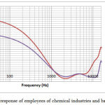Figure 1: Frequency response of employees of chemical industries and basketball players     Click here to View figure

The frequency response obtained was subjected to a statistical analysis. The results of the statistical analysis is depicted in Table 1

Table 1: Descriptive statistics for the FRT

	Chemical Industry				Basketball Players
Freq (Hz)	LF	NF	HF	EHF	LF	NF	HF	EHF
Mean	21.83	-4.14	0.72	14.15	15.45	-3.53	-5.27	-0.74
Median	19.46	-3.55	0.03	12.86	13.8	-3.4	-5.48	-3.29
Std Dev	13.67	1.9	3.11	4.76	9.64	1.29	0.64	5.75
Kurtosis	-1.01	3.63	9.65	22.69	92.96	1.66	0.41	33.03
Skew	0.43	0.33	0.44	0.39	0.42	1.15	0.74	0.62
Corr C-B	1	0.96	-0.89	0.98

From table 1, it is evident that at various frequency ranges, the response has varied. The frequency ranges were divided into 10 – 1000 Hz (Low Frequency – LF), 1010 – 6000 Hz (Normal Frequency – NF), 6010 – 10000 Hz (High Frequency – HF) and 10010 – 16000 Hz (Extended High Frequency – EHF) and the statistical parameters were obtained for these respective range of frequencies for both set of subjects.

The mean of the frequency response demonstrates a variation between the set sets of subjects in all the frequency ranges except NF. The mean value corresponds to the average response of the subjects at a given frequency range. A higher mean value indicates a lower perception of sound at a given range of frequency mean value of frequency response for employees of chemical industries at EHF is 14.15 dB). This is the main reason as to why the subjects seemed normal irrespective of their occupational background. Due to the absence of any kind of regular exposure to frequency ranges of LF and EHF, the subjects would have never realized these variations in their hearing perception. The variations in the mean frequency response in depicted in figure 2

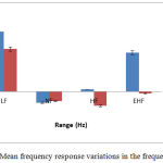Figure 2: Mean frequency response variations in the frequency range     Click here to View figure

The median corresponds to the central tendency, which is the location of the center of a group of numbers in a statistical distribution and denotes the central behavioral response for every frequency range with respect to the response of a given set of subjects and is given by figure 3. A lower median value corresponds to a better frequency response pattern denoting the betterment in the ability of the frequency response of the subjects. For instance, from figure 3, it is evident that the response of the basketball players in HF and EHF range is extremely better as compared to their counterparts (-5.48 dB and -3.29 dB respectively)

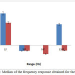Figure 3: Median of the frequency response obtained for the subjects     Click here to View figure

The standard deviation obtained denotes the variation of the response with respect to the average response value obtained. Hence it could be apt to regard a lower value to be better than a higher standard deviation value. The same is depicted in figure 4 from which it could be concluded that both NF and HF ranges have a lower deviation which proves the fact as to why subjects seem to be normal despite being from various backgrounds with respect to exposure. The response in NF and HF are similar in both the cases where lower values are observed as compared to the other frequency ranges (1.9 and 3.11 for chemical industry employees and 1.29 and 0.64 for basketball players). Also even in these range of frequencies, basketball players exhibit an excellent response with the least variation in the HF region as compared to their chemical counterparts proving a better response in this range

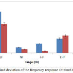Figure 4: Standard deviation of the frequency response obtained for the subjects     Click here to View figure

Kurtosis often measures the sharpness or flatness of a given distribution. In other word, this provides a measure about the tailedness of a given dataset. In convention, a normal distribution has a kurtosis value of 3. Positive value indicates a peaked distribution while a negative value indicates a relatively flat distribution. The kurtosis values obtained for the dataset is depicted in figure 5. From the results it is evident that the frequency response is relatively flat for both chemical industry employees as well as for the basketball players in the NF range (3.63 and 1.66 in NF). However, in the LF, although chemical industry subjects demonstrate a flat response, the basketball players show a highly peaked response (-1.01 and 92.96). But at the EHF, all the subjects have a peaked response (22.69 and 32.03). This indicates a similar response of both the categories of subjects in NF due to which the perception of sounds seem similar in both the cases. But at the LF and EHF, the peakness of the response rises providing an insight into the importance of LF and EHF in probing into the variations in the response characteristics of non-pathological subjects

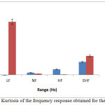Figure 5: Kurtosis of the frequency response obtained for the subjects     Click here to View figure

The skewness of the frequency response is obtained which characterizes the degree of asymmetry of a distribution around its mean. For the present results obtained, the skewness is positive indicating an asymmetric tail extending towards more positive values. Also the skewness is similar for both the sets of subjects in the LF (0.43 and 0.42) and the variations increase at the HF and EHF (0.44 and 0.74 in HF and 0.39 and 0.62 in EHF). But extreme variations are seen in the NF which hints at a possible usage of skewness to be a strong parameter to assess the variations between employees of chemical industries and the basketball players (0.33 and 1.15 in NF)

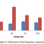Figure 6: Skewness of the frequency response     Click here to View figure

The correlation of a given two sets indicate the similarity between them. In other words, if this value of higher, a better correlation is seen and vice versa. For the present case, the correlation coefficients are obtained for the frequency response of the chemical industry employees and basketball players for the given frequency ranges. A pictorical depiction of the same is provided in figure 7 from which it is very evident that the frequency response in LF, NF and EHF (1, 0.96 and 0.98) although seem similar, there is a drastic variation between the frequency responses of the given two sets of data in HF range ( -0.89) and hence can be used as a strong feature to compare with each other

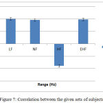Figure 7: Correlation between the given sets of subjects     Click here to View figure

Absolute Threshold Test (ATT) Results

As an extension, the intensity based variations were also obtained for the employees of chemical industries and compared against those of the basketball players. This test was run twice, once in the morning and again in the evening, as mentioned prior. The results obtained were subjected to a statistical analysis and the same is provided in table 2. The absolute threshold values obtained in the morning are depicted as CE and BE for chemical industry employees and basketball players respectively. Also for the evening test, the same is represented as CO and BO.

Table 2: Descriptive statistics for the absolute threshold test

	Chemical		Basketball
Absolute Threshold (dB)	CE	CO	BE	BO
Mean	39.54	49.07	49.24	44.13
Median	39.09	50.94	51.38	42.38
Std Dev	10.44	13.35	13.52	12.82
Kurtosis	-1.12	-0.94	-0.56	-0.53
Skew	0.12	-0.38	-0.4	0.32
Correlation (E:O)	-0.18		0.63
Correlation (E:E)	0.16
Correlation (O:O)		-0.37

The mean value of the absolute threshold surprisingly demonstrate a better perception of the intensity in the employees of chemical industries in the morning test, as compared to the basketball players (39.54 and 49.24 dB). But as the day progresses, the employees are exposed to various solvents and the basketball players would have spent their day with conventional activities including practicing / training in their sport. So, by the evening, the mean perception value would have reduced in case of chemical industry employees and increased in case of basketball players as expected (49.07 and 44.13 dB). This shows a decrease in the perception by 9.76 dB in case of employees and improvement by 4.94 dB in case of basketball players by the end of their routine. Figure 8 depicts the variations in the mean absolute threshold value

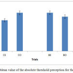Figure 8: Mean value of the absolute threshold perception for the subjects     Click here to View figure

The median of the absolute threshold values obtained show a distinct pattern with respect to improvement / deterioration of the absolute threshold. While it is evident that the day progresses in cases of chemical industry employees and vice versa for basketball players, the median too behaves in a similar manner. While the median value is less for CE and BO (39.09 and 42.38 dB), it increases for CO and BE (50.94 and 51.38 dB) indicating that a lower median value corresponds to a better auditory threshold in human beings

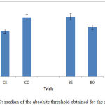Figure 9: median of the absolute threshold obtained for the subjects     Click here to View figure

The standard deviation too behaves similar to the median with a lower value for CE and BO (10.44 and 12.82 dB) and vice versa for CO and BE (13.35 and 13.52 dB)

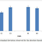Figure 10: standard deviation observed for the absolute threshold values     Click here to View figure

The kurtosis values obtained clearly indicate a flat distribution for all the sets of subjects thereby not providing a variation in the flatness of peakness of the values obtained. However, one could conclude that the kurtosis values for the chemical industry employees are more peaked (-1.12 and -0.94) while the peakness is lesser in case of basketball players (-0.56 and -0.53).

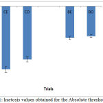Figure 11: kurtosis values obtained for the Absolute threshold values     Click here to View figure

The skew values obtained provide a clear differentiation with respect to improvement / deterioration of the absolute threshold values. While the Absolute threshold deteriorates for chemical industry employees, the skewness drastically varies from a positive value to a negative value (0.11 and -0.38). in case of basketball players, the pattern is exactly reversed in terms of the improvement of the absolute threshold value and the skewness value too behaves in a similar manner (-0.4 and 0.32). This indicates a transition in the skewness from an asymmetric tail extending towards more positive values to more negative values in the dataset

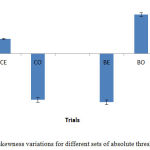Figure 12: skewness variations for different sets of absolute threshold values     Click here to View figure

Figure 13 depicts a correlation performed between various sets of data obtained. While CE and CO results are negatively correlated, indicating the difference in the readings (-0.18), the BE and BO values are positively correlated hinting the presence of a similarity in the data patterns in case of basketball players in the morning asnd in the evening tests (0.63). but this similarity is reduced in case of morning values as compared with chemical and basket ball players (0.16), the exit values of chemical industry employees and basketball players are negatively correlated (-0.37). this indicates that the CE:CO and CO:BO are negatively correlated which is as expected due to the fact the absolute threshold values deteriorate as the day progresses in case of employees of the chemical industries and improve in case of basketball players

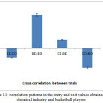Figure 13: correlation patterns in the entry and exit values obtained for chemical industry and basketball players     Click here to View figure

Based on the results depicted in this section, one could conclude that absolute threshold can be quantified with the aid of statistical analysis. It is also evident that the absolute threshold deteriorates in case of employees of chemical industries before and after their work while it improves in case of basketball players providing substantial proof for the effects of undesired conditioning and desired conditioning respectively. A similar analysis could be made in case of other industries with occupational exposure and hence a comparison can be possibly made with the human beings exposed to various types of occupational noise in order to assess the psychophysical variations with the aid of the perception of auditory temporal resolution. Also as seen in case of basketball players, professional players into more sports such as cricket and table tennis could be included in this research in order to be able to compare between different sports for the assessment of variations in desired conditioning as well

Acknowledgements

The authors wish to thank Jain University for providing a constant support during the present work. Also credits to Centre for Medical Electronics Research, MSRIT for helping with data collection. The analysis of the data has been conducted with the aid of MedNXT Innovative Technologies, Bangalore. The authors wish to thank them as well. MATLAB based tools such as Hearing Test tool (Developed by Dr Samir Rawashdeh) and psychoacoustics toolbox (developed by Dr Massimo Grassi) have been used for the present work.

Funding Source

Also the authors hereby clarify that there is no financial interest associated with this work

Conflict of Interest

The authors also wish to hereby declare that there is no conflict of interest of any kind regarding the publication of this paper.

References

1. Theunissen, Frédéric E., and Julie E. Elie. “Neural processing of natural sounds.Nature Reviews Neuroscience. 2014;15(6):355-366.
   CrossRef
2. Greta C. S and Johnson A. T. Auditory function in normal-hearing, noise-exposed human ears. Ear and hearing. 2015;36(2):172.
3. Donald J. L and Phelps A. R. Health Is More than Medicine. Health Care for People with Intellectual and Developmental Disabilities across the Lifespan. Springer International Publishing. 2016;15-29.
   CrossRef
4. Seunghee H., et al. In-Vehicle System Design-Considering Cognitive Characteristics of Elderly Drivers.Platform Technology and Service (PlatCon), 2017 International Conference on. IEEE. 2017.
   CrossRef
5. Thomas S., et al. Technological advancements in sport psychology. Routledge Companion to Sport and Exercise Psychology: global perspectives and fundamental concepts. 2014.
6.  Boris G., et al. “Is the din really harmless? Long-term effects of non-traumatic noise on the adult auditory system.” Nature Reviews. Neuroscience. 2014;15(7):483.
7.  John M. L., et al. “Hearing loss: diagnosis and management.” Primary Care: Clinics in Office Practice. 2014;41(1):19-31.
   CrossRef
8. Michael A. S and  Moore C. J. B. Amplitude-modulation detection by recreational-noise-exposed humans with near-normal hearing thresholds and its medium-term progression. Hearing research. 2014;317:50-62.
   CrossRef
9. Alessandro S and Grassi M. “PSYCHOACOUSTICS a comprehensive MATLAB toolbox for auditory testing.” Frontiers in psychology. 2014;5.
   CrossRef
10. Giovanna M., et al. The impact of a concurrent motor task on auditory and visual temporal discrimination tasks. Attention, Perception & Psychophysics. 2016;78(3):742-748.
    CrossRef
11. Pierre C ., Morata C. T and Hong O. Chemical exposure and hearing loss. Disease-a-month: DM. 2013;59(4):119.
12.  Toni H., et al. Context-dependent sound event detection. EURASIP Journal on Audio, Speech, and Music Processing. 2013;2013(1): 1.
13.  John P., Villota K., et al. Augmented Reality for Improved Dealership User Experience. No. 2017-01-0278. SAE Technical Paper. 2017.
14. Curtis J. B., et al. Electrophysiology and Perception of Speech in Noise in Older Listeners: Effects of Hearing Impairment and Age. Ear and hearing. 2015;36(6):710-722.
    CrossRef
15.  Simone S., et al. “Effects of stimulus order on auditory distance discrimination of virtual nearby sound sources. The Journal of the Acoustical Society of America. 2017;141(4):375-380.
    CrossRef
16.  Alice C., et al. Auditory abilities of young adults, middle-age adults and old adults. Giornale italiano di psicologia. 2015;42(1-2):249-262.
17. Elena F., et al. Rhythm perception and production predict reading abilities in developmental dyslexia.” Frontiers in human neuroscience. 2014;8
    CrossRef
18. Christopher J. P.Daphne Barker, and Garreth Prendergast. “Perceptual consequences of “hidden” hearing loss. Trends in hearing. 2014;18:2331216514550621.
    CrossRef
19.  Leah F., Ben-Artzi E and  Babkoff H. Aging and speech perception: Beyond hearing threshold and cognitive ability. Journal of basic and clinical physiology and pharmacology. 2013;24(3):175-183.
    CrossRef
20.  Qiao H., et al. Voluntary movement affects simultaneous perception of auditory and tactile stimuli presented to a non-moving body part.Scientific reports. 2016;6:33336.
    CrossRef

(Visited 485 times, 1 visits today)