Pratima Purushottam Gumaste^*and Vinayak K. Bairagi

Department of Electronics and Telecommunication, AISSM’s Institute of Information Technology, Savitribai Phule Pune University, Pune, India.

Corresponding Author E-mail : pratimagumaste@gmail.com

DOI : https://dx.doi.org/10.13005/bpj/1871

Abstract

Brain tumors vary in their position, mass, nature, and consistency of these lesions. Due to the similarities found between brain lesions and normal tissues, many challenges are faced by the researcher in developing algorithms for tumor segmentation. Brain tumor abstraction is thought-provoking job in medical image handing out because brain image and its structure is complicated. Segmentation plays a vibrant role in processing of medical images. Magnetic Resonance Imaging has become a particularly useful medical diagnostic tool for diagnosis of brain and other medical images.The objective of this paper is to develop an algorithm that facilitates the study of feature extraction from the brain right and left hemispheres. The proposed study, also highlight a completely different advanced higher order statistical features extracted from the chosen region of brain slice. The tumor area is extracted from statistical features using Support Vector Machine.  The proposed methodology can be used to locate tumor tissues based on a single-spectral structural Magnetic resonance image.

Keywords

Benign Tumor; Gray Level Cooccurrence Matrix; Magnetic Resonance Imaging (MRI); Statistical Features; Textural Features; T₂ Weighted Images.

Download this article as: 

Copy the following to cite this article: Gumaste P. P, Bairagi. V. K. A Hybrid Method for Brain Tumor Detection using Advanced Textural Feature Extraction .Biomed Pharmacol J 2020;13(1).

Copy the following to cite this URL: Gumaste P. P, Bairagi. V. K. A Hybrid Method for Brain Tumor Detection using Advanced Textural Feature Extraction . Biomed Pharmacol J 2020;13(1). Available from: https://bit.ly/2tnPRpK

Introduction

The brain is divided into two halves called the right and left hemispheres. The brain can also be divided into four areas known as lobes (frontal, temporal, parietal and occipital) plus two other important areas called the brain stem and the cerebellum. The presence of a brain tumour can cause damage to healthy brain tissue, disrupting the normal function of that area. A tumor formation takes place in the brain, due to the uncontrolled growth of cells. Brain tumors can be classified into two types such as a benign tumor (which does not spread cancer) or malignant tumor (which can spread cancer). Benign brain tumors have a homogenous structure that doesn’t contain cancer cells. These can be monitored radiologically or fully removed surgically. They won’t resurface. Malignant brain tumors are dissimilar in their structure, which results in cancer. Fig 1 a and b shows how the brain image looks with and without tumor.

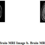Figure 1: a. Normal Brain MRI Image b. Brain MRI Image with Tumor Click here to View Figure

 

Brain tumors vary in features like dimension, outline, position, and image intensities. They may collapse adjacent structures. In the adults, glial tumors are the most common ones seen to be cancer-causing. They have a high rate of death. Glial tumors are observed in people with age group of 20 years and around. This type of the tumor covers about 90% of all types. The location of the growth of tumor is observed in the interstitial tissue cells of the brain. With the scaling, they disclose into the healthy brain tissues. Therefore, it is necessary to detect the brain tumor at the beginning stage itself.  So that further treatment method can be decided.  It can result in the protection of the life of the patient. It is important to detect Pathological brain from a normal brain. Physicians make decisions based on it, which helps avoid wrong judgments on subjects. In recent days, numerous imaging practices are seen. Magnetic resonance imaging (MRI) structures show a large number of details of soft tissues, spawning a corpus dataset. Brain pictures give indicators of brain composition. These details will be helpful in the analysis of the many brain abnormalities like malignant gliomas. There are basically three types of MRI images T₁ – weighted, T₂ – weighted and Flair. Tumors having similar options have a completely different look in T₁-Weighted, when put next to T₂ – Weighted and FLAIR ( Fluid-attenuated inversion recovery) MRI images (Chaddad and Tanougast. 2016). At present, many researchers are working on brain MR images for solving PBD [Pathological brain detection] problems. Computer-aided diagnosis (CAD) systems are currently available to identify unhealthy tissue from healthy brains and to classify severity degree (Zhang et al. 2015).

With the help of Image segmentation, an image is divided into smaller parts called modules or subsets. This division of image is performed based on one or more characteristics or features. Segmentation enhances areas of interest.   The image segmentation can be manual or automatic. Manual segmentation of MR images in the brain may be a time consuming and tedious process. It is quite possible that the result obtained may be different when a different specialist performs the activity. For doing the segmentation of 500-2000 brain images sized 512 * 512, experts need around 2-4 hours. Also, there is 14% – 22% differences in the remarks obtained from person to person. For physicians, dynamic computerized segmentation is of great help. Large dataset analysis and diagnosis is of brain diseases in a quantitative means are possible due to this method. However, segmentation of the brain tissues may be a quite troublesome task. The non-uniform intensity in a division, surrounding noise, complex shape, indistinct borders are some of the reasons for this ( Demirhan, Mustafa and Guler. 2015). Hence there is still scope to improve upon the segmentation algorithms.

The proposed algorithm is developed with extraction of features using advanced higher order statistical features to detect the tumor portion. Also, SVM classifier is used to authenticate the presence of a tumor in the input images. The remaining paper is organized as Section II briefs the trends in the algorithms developed in Brain tumor detection, Section III discusses our detailed proposed technique with material and methods. Section IV highlights the results and discussion of proposed method and Section V includes conclusion and further future scope of  the proposed work.

Literature Survey

Researchers have proposed different systems in the literature for the identification of the region of interest. There can be inherent difficulty in the detection and quantification of the brain tissues in Brain MR Images. There has always been a challenging task needed for the purpose of diagnosing brain tumors and other neurological diseases (Demirhan, Mustafa and Guler 2015).

These methods consist of thresholding of an image and performing morphological techniques, applying the watershed method, opting for region growing approach, doing asymmetric analysis, atlas-based approach, outline/plane evolution method, supervised and unsupervised learning methods. Segmentation of images is done based on intensity through the approaches like thresholding; edge detection and morphological operation. Segmentation performance relies on the differentiation between the intensities among the tumor and non-tumor regions. Also, watershed and region growing techniques are effortless but are sensitive to noise. This is the drawback of intensity-based approaches. The normal or healthy brain exhibits largely symmetric property. So, one can divide the brain into two hemispheres. Further, this can also improve the tumor identification and segmentation process because tumor segmentation can be done only in half section of the hemisphere. The limitation of this technique is computations. Iterations remain the same as other methods when a tumor is located across mid-sagittal plan. Atlas-based methods measure the dissimilarity between irregular and regular brain images.

Table 1 summarizes some of the recent works and its methodology and findings. The research conducted in Brain Tumor detection still has some limitations and challenges. To raise the reliability of the classification it should be tested for a determined number of recital constraints. In order to achieve good exactness, sensitivity, and specificity, more features need to be considered but for optimized, less computation and good performance system selective features are useful.

Table 1: Summary of recent work

Sr. No.	Authors with year of Publication	Methodology	Performance Parameters
1	(Alexis Arnaud et al, 2018)	Probabilistic mixtures Discriminative multivariate features, Fingerprint model	MRI data collected in rats bearing a brain tumor have been processed
2	(Sayd Tahri Yassine et al, 2018)	Nl-means filter, expectation maximization algorithm	Jaccard Similarity Coefficient = 0.90 Dice Similarity Coefficient metric = 0.88 Sensitivity = 0.81 Specificity = 0.85
3	(Zhenyu Tang et al, 2018)	multi-atlas segmentation (MAS) framework a new low-rank method SCOLOR	Recovering normal brain appearances from tumor regions while also preserving normal brain structures. To improve the accuracy of brain functional connectivity networks (FCN)
4	(Daniele Ravi et al, 2017)	Dimensionality reduction extension of the t-SNE Semantic Texton Forest (STF)	Specificity = 86.57 Sensitivity = 86.88
5	(Wang Mengqiao et al, 2017)	22-layers deep, three dimensional Convolutional Neural Network (CNN), N4ITK,	Dice Similarity Coefficient metric 0.84, Positive Predictive Value 0.88 and Sensitivity 82
6	(Sergio Pereira et al, 2016)	Convolutional Neural Networks (CNN)	Dice Similarity Coefficient metric (0.88, 0.83, 0.77) for BRATS 2013 Database
7	(K. Bhima & A. Jagan, 2016)	Watershed Method, Marker-based Watershed Image Segmentation comparison	Different results obtained by researchers have been compared
8	(Aditi P. Killedar, Veena P. Patil & Megha S. Borse 2014)	Co-occurrence matrices, SVM	Clustering the abnormal images to detect two certain abnormalities
9	(Hussein Attya, Lafta Esraa and Abdullah Hussein, 2013)	gray-level co-occurrence matrix (GLCM) k-nearest neighbor (K-NN)	accuracy 88%.
10	(P. Shantha Kumar & P. Ganesh Kumar, 2010)	Grey level and wavelet features Support vector machine	Sensitivity 99.4% Specificity 99.6% Positive predictive value 97.03%
11	(Ananda Resmi S. & Tessamma Thomas, 2010)	First-order statistics, GLCM	descriptors are highly differentiable between low (grade I) and high grade (grade III) Glioma
12	(Xiaoou Tang, 1998)	A multilevel dominant eigenvector estimation algorithm	run-length matrices contain great discriminatory information
13	(Sahar Jafarpour, Zahra Sedghi & Mehdi Chehel Amirani, 2012)	GLCM features PCA+LDA, ANN KNN	low computational complexity and low computational time
14	(Ramadan M. Ramo, 2012)	snake algorithm and the second Fuzzy C-mean	snake method has high speed
15	(D. Jude hemanth, D. Selvathi & J. Anitha, 2009)	FCM and Modified FCM	modified FCM algorithm is a fast alternative to the traditional FCM
16	(Yusra Ibrahim Mohamed et al, 2013)	ANN Back Propagation	Accuracy 96.33%.
17	(Dr. M. Karnan & T. Logheshwari, 2010)	Ant Colony Optimization with Fuzzy segmentation	Finds the optimum label that minimizes the Maximizing a Posterior estimate to segment the image
18	(F Lanningham et al, 2006)	fractal-based texture features Self-Organizing Map, multi-layer feedforward neural network and SVM	With ANN (TPF) values is 75% to 100% SVM avg accuracy 95%

Material and Methods

Brain Magnetic Resonance Image [MRI] Dataset

An Open Access medical specialty Image program that has nearly 1,700,000 pictures from the open access set of PMC.(32) It even has over 7,400 chest x-rays from the American state University assortment. Further, open source pictures are shown in figure 2. From the literature survey, it has been observed that the MRI capturing can be done using MRI machines with different Field strength capacities. But Images captured with the 1.5 T field strength are generally used in the research work. This field intensity is sufficient to visualize the tumor in the images.

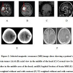Figure 2: Selected magnetic resonance (MR) image Click here to View Figure

Overview of the Proposed Method

The proposed automated brain tumor identification method go-through two-tier verification: initialization and fine-tuning authentication. Before doing this, for MRI artifact removal, images need to preprocess images using filtration. Two types of information are incorporated from MRI like intensity and spatial relationships of pixels to better the overall system performance. In phase one, proposed method detect and partition the MR images into two hemispheres based on the mutual information from histogram and symmetry analysis. Then, different statistical feature-sets are calculated in the “feature extraction technique” using texture analysis. Finally, the SVM classifier is used particularly for the brain tumor detection. In this step, based on first-order statistics and other features extracted from the target area, the classifier assigns a label to brain tissue. In the projected structure, the overall segmentation recital is improved with SVM classifier. A general outline of the proposed method is shown in Figure 3.

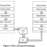Figure 3: Flow of Proposed technique Click here to View Figure

Feature Extraction

After region of interest has been extracted, its features are calculated in feature extraction step. A significant set of 32 intensity and grain textual features are extracted from the segmented Region of interest [SROI]. These features are First order Statistical Features, gray level co-occurrence matrix (GLCM), Grey Level Run Length Encoding Matrix (GLRLM), Grey Level Gap Length Matrix (GLGLM) and Grey Level Size Zone Matrix (GLSZM).

The features extracted in the current work and their fundamentals are discussed below: All these give us some relevant information regarding the texture of the image. Formulas for these features are listed below:

The first order statistical features

First order applied mathematics features: Mean, average distinction, energy, and entropy, lopsidedness and kurtosis square measure are the helpful first-order applied mathematics options.

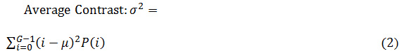
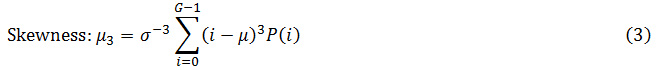
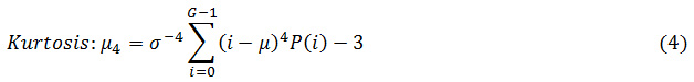
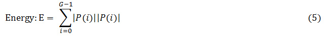
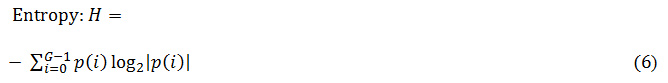
Where G is the maximum gray level of the image and P(i) is the probability density of the intensity levels which are obtained from:

Where h(i) is the total number of pixels with intensity level (i) and N is the total number of pixels in the image.

Grey Level Co-occurrence Matrix Features

The GLCM may be a second bar chart that describes the prevalence of pairs of pixels that are separated by a precise distance, d. Let I (x, y) be a picture with size NXM, and with G grey levels, and (x₁,y₁) and (x₂, y₂) be 2 pixels with grey level intensities i and j, severally. Once taking ∆x= x₂-x₁ within the x-direction and ∆y = y₂ – y₁ in the y-direction, the connecting line contains a direction θ that is adequate arctan(∆y/∆x). The normalized co-occurrence matrix Cθ;d is outlined as:

Here, A may be a given condition, like (∆x=d sin θ), (∆y=d cos θ), (I (x₁, y₁) =i), and (I (x₂, y₂) =j). Further on, NUM represents the variety of components within the co-occurrence matrix and K is the total variety of pairs of pixels. Normally, d = 1, 2 and θ = 0⁰, 45⁰, 90⁰, 135⁰ are used for calculation. Eight totally different texture options are

outlined with victimization co-occurrence matrix as follows

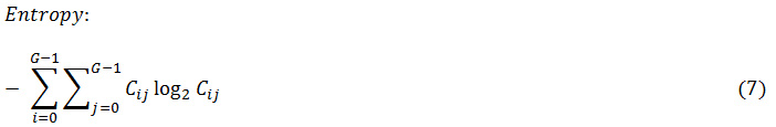
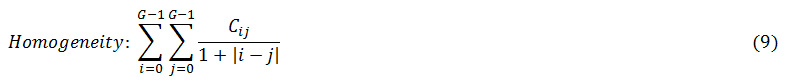
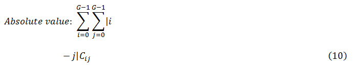
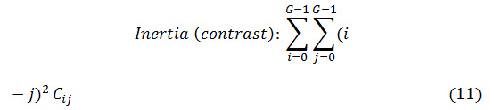
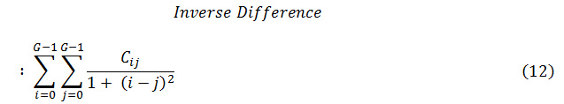
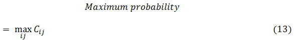
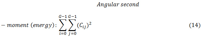
Where C_ij is the (i, j) ^th element of the co-occurrence matrix.

Grey Level Run Length Method Features

The grey level runs area unit characterized by the length and direction of specific gray price. To calculate GLRLM, the quantity of grey level running of varying lengths should be discovered. within the grey level run length matrix of R(θ) = [r’(i, l|θ)], the component r’(i, l|θ) provides associate degree estimate of the quantity of times which a picture contains a run with a length of  l, for a grey level i, within the direction of angle θ. the grey level run length matrices R(θ) area unit calculated for are 0⁰,45⁰, 90⁰ and 135⁰.The following five GLRLM features which are calculated using these matrices

SRE: Short Run Emphasis

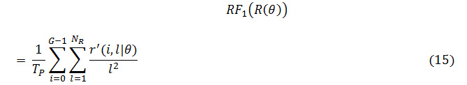
LRE: Long Run Emphasis

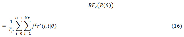
GLD: Gray Level Distribution

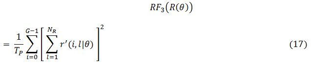
RLD: Run-length Distribution

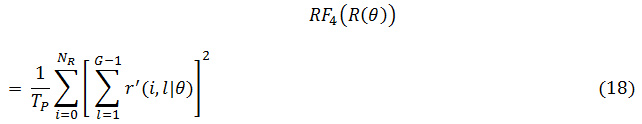
RP: Run Percentage

In which G is the number of gray levels, N_R is the number of run lengths in the matrix, and T_P is

Grey Level Size Zone Matrix

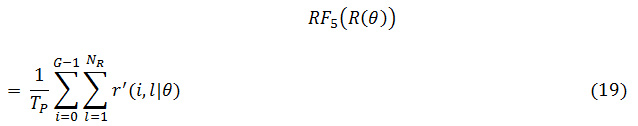
The starting lines of Thibault matrices are the grey level Size Zone Matrix (SZM). For a texture image f with N grey levels, it’s denoted with GSf (s, g) and provides an applied mathematical illustration by the estimation of a quantity with contingent probability density to perform the image distribution values. Its calculation is consistent with the pioneering Run Length Matrix principle: the worth of the matrix GSf (s, g) is adequate the quantity of zones of size s and of grey level g. The ensuing matrix encompasses a mounted range of lines adequate N, the number of grey levels, and a dynamic range of columns, which are determined by the scale of the most important zone in addition to the size of the division.

The more the additional solid thing they feel, the broader the matrix is going to be. This matrix has the advantage of not requiring calculations in many directions as that area unit is replaced by tagging the totally different areas. However, specifying the number of grey levels continues to be necessary, yet this renders the calculations strong in relation to noise. The eleven same indexes for the Run Length Matrix are often calculated. (Ramadan M. Ramo, 2012), (J. Anitha, D. Jude hemanth & D. Selvathi, 2009). SZM doesn’t need computation in many directions, contrary to RLM and co-occurrences matrix (COM). However, it’s been by trial and error test that the degree of grey level division still has a crucial impact on the feel classification performance. For a general application, it’s typically needed to check much grey level division so as to search out the best one with regard to a coaching dataset. By trial and error, “thirty-two” typically provides the simplest result.

More exactly, this matrix is especially economical to characterize the feel homogeneity, non-cyclist or speckle-like texture; it has provided better characterization than granulomere (or COM, RLM, etc.) for the classification of cell nuclei, dermis, road quality (bitumen condition) and a few textures in PET pictures. In fig 4 given below sample image and its grey level size zone feature matrix calculation is demonstrated.

Figure 4: (a) Sample Input Image (b) Corresponding Click here to View Figure

Two class separations of data points are possible with it. Image classification, image recognition, and bioinformatics are the areas in which SVM can be applied. It is doing well as it comes up with the sensible classification which leads to numerous application domains, e.g. diagnosing. The principal of operating of SVM is the structural- risk- decrease- technique from the applied math- learning theory. Given a collection of coaching examples, associate SVM coaching formula builds a model that assigns new examples into one class or the opposite, creating it a non-probabilistic binary linear classifier. In addition to playing linear classification, SVMs will efficiently perform non-linear classification victimization what is referred to as the kernel trick, implicitly mapping their inputs into high-dimensional feature areas. From a given category in an exceedingly high dimension feature house, a support vector machine identifies associate and best separating hyperplane between members and non-members of a given set. The entry purpose of the SVM formula is to see the characteristics in terms of a feature set from information pre-processing step and extracted victimization having completely different matrices methodology. In planned methodology, the SVM is employed to differentiate between pictures with tumors and those not having tumor categories.

Results and Discussion

The tumour identification from a imaging could be a advanced method hence computing is useful to notice the precise tumor position during a brain imaging. In this work we tend to develop a unique technique for the tumor segmentation from 2D images. The deliberate technique is in detail represented within the preceding Section III and during this section the detail clarification on the execution result and its performance is analyzed. The projected approach for the brain tumor is prescribed in the operating platform of MATLAB and also the elaborate clarification on the implementation performance is as follows.

The following images represent the results obtained from the proposed algorithm. Fig 5(A), (B) and (C) gives an idea about the GUI developed, selected hemisphere and the obtained output respectively.

Figure 5: (A) Developed Graphical User interface [GUI]  (B) Selected hemisphere  (C) Obtained output Click here to View Figure

In fig 6, we illustrate the basic results obtained for the brain partitioning and the obtained histograms for a case I and case II.   Also, it depicts the difference in the histogram obtained shows the pick value for brain MRI with a tumor case. In both the Cases  1 and 2 a pick is observed, when difference between right and left brain hemisphere histogram is plot. This pick indicates the asymmetry present in the two halves of the brain. This asymmetry indicates the abnormality present on one of the side of the brain. But, when the difference histogram is plotted for normal brain, pick height is observed very minor and can be neglected.

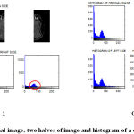Figure 6: Histogram of an original image, two halves of image and histogram of a difference image of case 1 and 2 Click here to View Figure

 

A set of features obtained from proposed methodology

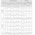Table 2a: Statistical Features obtained for Images both from with tumor and without tumor cases. Click here to View Table

 

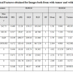Table 2b: Statistical Features obtained for Images both from with tumor and without tumor cases. Click here to View Table

Comparison of the Result

The above Table 2.a and Table 2.b illustrates the details of the features obtained from the statistical analysis of the MRI images with normal brain images and images with a tumor. From the results obtained it is seen that the out of obtained features Average Contrast and Mean from first-order statistical feature set and Homogeneity, Absolute Value, Inertia Contrast from second-order statistical feature set i.e. GLCM features shows a remarkable difference for normal and with tumor images.

Table 3: Methods Used in Literature and their findings

Sr. No.	No of Images	Method Used	Avg Accuracy	Result
1	334	FCM	92.55	Modified Convergence rate observed is superior [21]
		Modified FCM	92.45
2	–	ACO	80	ACO with FCM performs better [23]
	–	ACO with Fuzzy	92
3	204	SVM	91%	–
4	100	SVM (Proposed Algorithm)	92.60	Average Time required is reduced

While observing the results obtained by other researchers, the experimentation is done on the BRATs database. This database includes the simulated images of brain. But, when experimentation in our proposed work is done on online images, results are a bit lowered.

Comparison of Results in Terms of Execution Time Required

Table 4: The Result obtained by researchers available in the literature

Sr. No.	No. of Samples used	Method 1	Method 2	Comparison of Avg. Time required
1	4	Snake Algorithm	Fuzzy Method	Method 1 Requires less time [19]
2	30 and more	Proposed method		Works on the half part hence execution time gets reduced still.
3	–	ANN		0.2434 sec. [19]

In the literature work the existing algorithms extracts the features from entire brain image. Hence, algorithm needs more iterations to executes.    The proposed algorithm initially choose the correct half for the feature extraction. After this step, it extracts the statistical features from the selected half portion of the brain. Computational time needed are compared in the Table 4. 

Conclusion

There are many method segmentation algorithms present in the literature. Each one has its superior points and drawbacks depending on the methodologies used, screening techniques used(i.e. CT scan, MRI). The proposed algorithm divides the 2D MRI images into two hemispheres left and right. Statistical features are extracted from the selected half portion of the brain MRI by. Among the features extracted from the image, it has been observed that Mean, Homogeneity, Absolute Value, Inertia, Contrast, Average Contrast, LRE, GLD, RLD, Variance are prominent ones. The SVM is used as a classifier. As the size of the image increases, it leads to increased computations to detect the tumor. This increased time for detection may not be acceptable in critical cases. This proposed approach of slicing brain into two halves for Brain Tumor Detection from MRI Images will have better computational efficiency compared to other methods as it only processes half section of the image. The execution time of the algorithm also gets reduced, but its efficiency is retained. The implemented algorithm is applicable to axial and Coronal slice images only due to the symmetry property of the brain. In future, the prosed algorithm need to be applied on the simulated images so that obtained results can be authenticated precisely.

Acknowledgements

This works is was not supported by research grants.

References

1. V. Anitha, S. Murugavalli. Brain tumor classification using two-tier classifier with adaptive segmentation technique. IET Computer Vision. 10 (1), 9–17 (2016).
2. Ayse Demirhan, Mustafa, Inan Guler. Segmentation of Tumor and Edema Along with Healthy Tissues of Brain Using Wavelets and Neural Networks. IEEE Journal of Biomedical and Health Informatics. 19 (4), 1451-1458 (2015).
3. Yu‑Dong Zhang, Shui‑Hua Wang, Xiao‑Jun Yang, Zheng‑Chao Dong, Ge Liu, Preetha Phillips and Ti‑Fei Yuan. Pathological brain detection in MRI scanning by wavelet packet Tsallis entropy and fuzzy support vector machine. Springer Plus. 4 (716), 712–716 (2015).
4. Ahmad Chaddad, Camel Tanougast. Quantitative evaluation of robust skull stripping and tumor detection applied to axial MR images. Brain Informatics. 3 (1), 53–61 (2016).
5. Meiyan Huang, Wei Yang, Yao Wu, Jun Jiang, Wufan Chen, Qianjin Feng. Brain Tumor segmentation Based on Local Independent Projection-Based Classification. IEEE Transaction on Biomedical Engineering. 61(10), 2633–2645 (2014).
6. Dongjin Kwon, Marc Niethammer, HamedAkbari, Michel Bilello, Christos Davatzikos and Kilian M. Pohl. PORTR: Pre-Operative and Post-Recurrence Brain Tumor Registration. IEEE Transactions on Medical Imaging. 13(3), 651-667 (2014).
7. Arshad Javed, Abdul hameed Rakan Alenezi1, Wang Yin Chai, Narayanan Kulathuramaiyer. Diagnosis System for the Detection of Abnormal Tissues from Brain MRI. Life Science Journal. 10(2), 1949–1955 (2013).
8. Atiq Islam, Syed M. S. Reza, and Khan M. Iftekharuddin. Multifractal Texture Estimation for Detection and Segmentation of Brain Tumors. IEEE Transactions on Biomedical Engineering. 60(11), 3204–3215 (2013).
9. Stefan Bauer, Christian May, Dimitra Dionysiou, Georgios Stamatakos, Philippe Buchler, and Mauricio Reyes. Multiscale Modeling for Image Analysis of Brain Tumor Studies. IEEE Transactions On Biomedical Engineering. 59(1), 25 – 29 (2012).
10. Shaheen Ahmed, Khan M. Iftekharuddin, and Arastoo Vossough. Efficacy of Texture, Shape, and Intensity Feature Fusion for Posterior-Fossa Tumor Segmentation in MRI. IEEE Transactions on Information Technology in Biomedicine. 15 (2), 206–213 (2011).
11. Albregtsen, F. Statistical Texture Measures Computed from Gray Level Co-occurrence Matrices. Image Processing Laboratory Department of Informatics. University of Oslo: University of Oslo, 1-14 (2008).
12. Gadkari, Dhanashree, Image Quality Analysis Using GLCM. M.S,. Florida, Orlando: University of Central Florida (2004).
13. Megha S. Borse, Aditi P. Killedar Veena P. Patil. Content Based Image Retrieval Approach to Tumor Detection in Human Brain Using Magnetic Resonance Image. In 1st International Conference on Recent Trends in Engineering & Technology. Nasik, 24 & 25 March. IEEE. 211-214 (2012).
14. Hussein Attya Lafta Esraa Abdullah Hussein. Design a Classification System for Brain Magnetic Resonance Image. Journal of Babylon University, Pure and Applied Sciences. 21(8), p.1-8 (2013).
15. P. Shantha Kumar and P. Ganesh Kumar. Performance Analysis of Brain Tumor Diagnosis Based on Soft Computing Techniques. American Journal of Applied Sciences . 11(2), p. 329-336 (2014).
16. Ananda Resmi S., Tessamma Thomas. Texture Description of low grade and high-grade Glioma using Statistical features in Brain MRIs. ACEEE, IJRTET. 4(3), 27-33 (2010).
17. Xiaoou Tang. Texture Information in Run-Length Matrices. IEEE Transactions On Image Processing. 7(11), 1602-1603 (1998).
18. Sahar Jafarpour, Zahra Sedghi, Mehdi Chehel Amirani. A Robust Brain MRI Classification with GLCM Features. International Journal of Computer Applications. 37(12), 1-5 (2012).
19. Ramadan M. Ramo. Brain Tumor Detection Using Snake Algorithm and Fuzzy C-Mean. Raf. J. of Comp. & Math’s.. 9(1), 85-100 (2012).
20. J. Anitha, D. Jude hemanth, D. Selvathi. Effective Fuzzy Clustering Algorithm for Abnormal MR Brain Image Segmentation. International Advance Computing Conference. Patiyala, 6-7 March 2009. IEEE: IEEE. 609-614 (2009).
21. Yusra Ibrahim Mohamed, Walaa Hussein Ibrahim, Ahmed Abdelrahman Ahmed Osman. MRI Brain Image Classification Using Neural Networks. In International Conference on Computing, Electrical and Electronics Engineering. Khartoum, Sudan, 26 – 29 August. IEEE: IEEE. 253-258 (2013).
22. Dr. M. Karnan, T. Logheshwari. Improved Implementation of Brain MRI image Segmentation using Ant Colony System. In International Conference on Computational Intelligence and Computing Research. Coimbatore, India, 28-29 Dec 2010: IEEE. 1-4 (2010).
23. F Lanningham, KM Iftekharuddin, J Zheng, MA Islam, RJ Ogg. Brain Tumor Detection in MRI: Technique and Statistical Validation. In Fortieth Asilomar Conference on Signals, Systems and Computers. Pacific Grove, CA, USA, 29 Oct.-1 Nov. 2006. IEEE: IEEE. 1983-1987 (2006).
24. Alexis Arnaud, Florence Forbes, Nicolas Coquery, Nora Collomb, Benjamin Lemasson, and Emmanuel L. Barbier. Fully Automatic Lesion Localization and Characterization: Application to Brain Tumors using Multiparametric Quantitative MRI Data. IEEE Transactions on Medical Imaging. 37(7), 1678-1689 (2018).
25. R. Abdelilah, S. T. Yassine, S. Sara, C. Bouchaib. A new fast brain tumor extraction method based on Nl-means and expectation maximization. In International Conference on Optimization and Applications. Mohammedia, Morocco, 26-27 April 2018. IEEE: IEEE. 1-5 (2018).
26. Tang, Z., Ahmad, S., Yap, P. T., & Shen, D. Multi-Atlas Segmentation of MR Tumor Brain Images Using Low-Rank Based Image Recovery. IEEE Transactions on Medical Imaging. 37(10), 2224-2235 (2018).
27. Ravì, Daniele & Fabelo, Himar & Marrero Callico, Gustavo & Yang, GuangZhong. Manifold Embedding and Semantic Segmentation for Intraoperative Guidance With Hyperspectral Brain Imaging. IEEE Transactions on Medical Imaging. 10(19), 1-10 (2017).
28. Wang Hao, Wang Mengqiao, Yang Jie, Chen Yilei. The Multimodal Brain Tumor Image Segmentation Based on Convolutional Neural Networks. In International Conference on Computational Intelligence and Applications. Beijing, China, 8-11 September. IEEE: IEEE. 336-339 (2017).
29. Sergio Pereira, Americo Oliveira, Victor Alves and Carlos A. Silva. On Hierarchical Brain Tumor Segmentation in MRI Using Fully Convolutional Neural Networks: A Preliminary Study, IEEE 5^th Portuguese Meeting on Bioengineering (ENBENG), 16-18 February. IEEE. 1–4 (2017).
30. Sergio Pereira, Adriano Pinto, Victor Alves, and Carlos A. Silva. Brain Tumor Segmentation Using Convolutional Neural Networks in MRI Images. IEEE Transactions on Medical Imaging. 35(5), 1240–1252 (2016).
31.  K. Bhima, A. Jagan. Analysis of MRI based Brain Tumor Identification using Segmentation Technique. An International Conference on Communication and Signal Processing, April 6-8, 2016, 2109–2113 (2013).
32. NLM/NIH. Open Access Biomedical Image Search Engine. [ONLINE] Available at: https://openi.nlm.nih.gov/. [Accessed 1 March 2019]. 2019.

(Visited 2,339 times, 2 visits today)