
Manuscript accepted on :06-10-2025
Published online on: 21-10-2025
Plagiarism Check: Yes
Reviewed by: Dr. Nagham Aljamali and Dr. Gheri Febri Ananda
Second Review by: Dr. Amna Iqbal
Final Approval by: Dr. Kapil Joshi
Mohammed Muddasir Naseer1 , Veeraprathap Veerabhadraiah2, Basavaraj Rayappa Ramji3, Santhosh Kumar Kadur Lokeshappa4, Srividya Chandagirikoppal Nagendra5, Yathiraj Guduganahalli Ramesh6 and Kiran Puttegowda7*
1Department of ISE, Vidyavardhaka College of Engineering, Mysuru, Karnataka, India
2Department of ECE, ATME College of Engineering, Mysuru, Karnataka, India
3Department of Industrial Engineering and Management, BMS College of Engineering, Bangalore, Karnataka, India
4School of Computer Science and Engineering, Presidency University, Bengaluru, Karnataka, India
5Department of ECE, BGS Institute of Technology, Adichunchanagiri University, Karnataka, India
6Department of CSE (Cyber Security), Coorg Institute of Technology, Ponnampet, Karnataka, India
7Department of ECE, Vidyavardhaka College of Engineering, Mysuru, Karnataka, India
Corresponding Author E-mail: kiranhsn@vvce.ac.in
DOI : https://dx.doi.org/10.13005/bpj/3410
Abstract
Magnetic resonance imaging (MRI) is widely used for the non-invasive diagnosis of brain tumours; however, accurate manual interpretation remains challenging due to the complexity of tumour structures and inter-observer variability. In this study, we propose an optimized EfficientNet-B0 architecture for automated brain tumour detection and classification. Two models were developed: Model 1, trained from scratch, and Model 2, which integrated transfer learning, fine-tuning, and hyperparameter optimization. The models were trained and evaluated on a publicly available brain MRI dataset comprising four categories: glioma, meningioma, pituitary tumour, and no tumour. Model 1 achieved a testing accuracy of 94.52%, while Model 2 outperformed it with 99.43% accuracy, demonstrating superior generalization and stability. Comparative analysis with previous studies further confirmed that the proposed approach achieves higher accuracy and robustness in multi-class classification tasks. The results indicate that the optimized EfficientNet-B0 with transfer learning provides a reliable and effective framework for clinical decision support in brain tumour diagnosis.
Keywords
Accuracy; Brain Tumour Classification; Convolutional Neural Network (CNN); Deep Learning; EfficientNet-B0; MRI Image Analysis
Download this article as:| Copy the following to cite this article: Naseer M. M, Veerabhadraiah V, Ramji B. R, Lokeshappa S. K. K, Nagendra S. G, Ramesh Y. G, Puttegowda K. An Optimized EfficientNet-B0 Framework for Multi-Class Brain Tumour Detection and Classification from MRI Images. Biomed Pharmacol J 2026;19(June Spl Edition). |
| Copy the following to cite this URL: Naseer M. M, Veerabhadraiah V, Ramji B. R, Lokeshappa S. K. K, Nagendra S. G, Ramesh Y. G, Puttegowda K. An Optimized EfficientNet-B0 Framework for Multi-Class Brain Tumour Detection and Classification from MRI Images. Biomed Pharmacol J 2026;19(June Spl Edition). Available from: https://bit.ly/3WNuFU1 |
Introduction
A brain tumour is caused by the rapid growth of cells in the brain in an uncontrollable manner. Brain cancer accounts for approximately 1.3% of all cancer diagnoses in the US every year. All brain cancers are the result of a brain tumour, but not all brain tumours are cancerous. Non-cancerous tumours are labelled benign, while cancerous tumours are called malignant. The symptoms of having a brain tumour may vary depending on the location of the tumour growing inside the brain. Some of the common symptoms include seizures, behavioral or personality changes, progressive paralysis on one side of the body, and vision or speech problems.1 Although the causes of brain tumours remain unknown, there are a few factors that may increase the risk of developing a brain tumour. Some of these factors are exposure to excessive radiation, aging, and genetic conditions.2
Some of the common treatments of brain tumour include surgery, radiotherapy, chemotherapy, or a combination of any of these two, depending on the situation. However, these treatments do not guarantee the complete removal of the brain tumour. Conventional brain tumour treatment, like surgery is not effective against brain tumours that are located beyond the reach of a neurosurgeon. As for tumours that are located near the sensitive neural tissues, exposure to the radiation of chemotherapy is not feasible. Despite all this, early detection of the tumours followed by immediate treatment can significantly improve the chances of recovery of a patient.3,4
Fortunately, with the advancement in technology such as machine learning/artificial intelligence, the task of detection and classification of brain tumours can be made more effective and efficient. Presented in this assignment is a deep learning based model based on Convolutional Neural Networks (CNN) paired with a transfer learning approach to help detect the existence of brain tumour and further classify them into three types, namely glioma, meningioma, and pituitary tumour. Currently, a Magnetic Resonance Imaging (MRI) screening is the best way to detect brain tumours. However, due to the level of complexities involved in brain tumours and their properties, the identification of the type of brain tumours is complicated to begin with. Hence, a thorough analysis by professionals on the MRI images is required to determine whether the tumours are either malignant or benign. Occasionally, these manual examinations could be prone to error and bias, as different professionals have different points of view based on their own experiences. Also, the lack of medical professionals in developing countries makes it difficult and time-consuming to determine the properties of the brain tumour based on the MRI screening. Hence, an automated brain tumour detection and classification system can be developed using deep learning algorithms such as Convolution Neural Network (CNN) to assist medical practitioners in their brain tumour diagnosis and treatment plans.
This study is important because it produces an optimized EfficientNet-B0 model that improves precision, reliability, and extrapolation of brain tumour classification based on MRI scans. Compared to most previous studies, which concentrated on binary classification or demanded a lot of upfront preprocessing and large-scale calculations, the given method performs almost flawlessly (99.43% test accuracy) in a multi-class task with four different tumour types: glioma, meningioma, pituitary tumour, and no tumour. With these three strategies, dropout, adaptive learning rate scheduling, and transfer learning, the model can reduce overfitting and maintain consistent generalization with a relatively moderate-sized dataset. This compromise between the efficiency of computing and the accuracy of the diagnosis makes the framework a clinically suitable tool to support automated decision support, make fewer decisions based on the manual ones, and avoid the risk of wrong diagnosis. Moreover, the evidences of the improvements in comparison to baseline models and available literature highlight its novelty and the possibility of its practical implementation in healthcare systems, in general, and resource-limited settings, in particular, where timely and reliable diagnosis is of paramount importance. The Contributions of the Proposed Work are as follows.
Comprehensive Exploration of Deep Learning Architectures
The study conducts a detailed review and analysis of existing deep learning models specifically applied to brain tumour detection and classification using MRI data, highlighting their strengths and limitations.
Development of a Robust Classification Framework
A deep learning-based classification system is proposed using the EfficientNet-B0 architecture, capable of accurately detecting and classifying three major types of brain tumours—glioma, meningioma, and pituitary tumours—from MRI scans.
Performance Optimization through Fine-Tuning
The EfficientNet-B0 model is fine-tuned and optimized to achieve high classification performance, resulting in a significant improvement in accuracy, precision, recall, and F1-score, demonstrating its superiority over existing models such as WCNN and DeepTumourNet.
The structure of the article is as follows: the Section “Related work” is a brief description of the prior research. Section “Material and methods”: Presents the idea of the presented research and describes the distribution of data collected, model training, and its assessment. Section “Experimental results and discussion”: Discusses the obtained outcomes of the experiment and how they have been quantitatively and qualitatively assessed, using results from the simulation. Section “Conclusion and future work”: Summarizes the findings that have been presented at the end of the article and discusses the possibilities of further research.
Related works
In recent years, many researchers have ventured into machine learning, specifically deep learning techniques, to detect brain tumours and identify them as cancerous or benign. Deep learning architectures are preferred over traditional machine learning classifiers because the former are very robust in terms of feature extraction and are less time-consuming. In this section, some of the recent literature related to deep learning-based approaches for identifying and categorizing brain tumours is being discussed.
Qusay combined both ML and DL models to tackle both binary and multiclass classification issues, where the VGG16 architecture model demonstrated the best accuracy of validation and thus improved the reliability of the diagnosis.5 Vivek Kumar has shown that the Support Vector Machine (SVM) classification methods are sensitive to the identification of brain tumours in MRI scans, and this emphasises the significance of early diagnosis with the help of advanced image classification methods.6 Aditya Kumar reproduced the EfficientNet-B0 model and obtained 98% precision in identifying four types of tumours, including glioma, meningioma, pituitary, and non-tumour, thus confirming its usefulness as an automated selector.7 F. Abdullah compared custom CNN models and popular types of architectures such as DeepTumor-Net, VGG-16, ResNet-50, and Xception, producing very high accuracy with ResNet-50 and VGG-16 scoring 92.6 and 92.1 respectively.8 Anne Mary A has proposed a deep neural network (DNN) to segment tumour in MRI scans, which helps in improved diagnosis accuracy.9 In the same way, P. Vetrivelan applied CNN (CNN), VGG-16, or EfficientNetB3 in a dual-stage classification scheme that proved to be more capable of persistence and speed in diagnosing glioma, meningioma, and pituitary tumours.10 M.L. Sharma was aimed at the classification CNN of different types of tumours with metastatic tumours by paying attention to more effective decision-making at the clinical level.11 Mohammed Noori put forward a model based on ResNet50V2 and utilizing data augmentation and the model of class balancing, and demonstrated an accuracy rate of 95.29 percent.12 Mundru Navya Sree improved the classification using InceptionV3 and ResNet-50 architectures and preprocessing with adaptive median filtering and CLAHE.13 G Dilip Kumar tested the models of DenseNet-121, ResNet-101, and MobileNetV2, yielding a maximum accuracy of 99 percent with their best results using the DenseNet-121.14
Md Morsaline Billah combined classical image processing with VGG19 and InceptionV3 to achieve access to a validation of 100 percent.15 A hyperparameter-tuned CNN was used to obtain precision in tumour classification by Amita Banerjee as high as 94.82% with less use of expert advice.16 A Soheil Saeedi compared several ML methods and developed a CNN-based architecture and an autoencoder architecture with respective yields of 96.47 and 95.63 percent in detecting three tumour types.17 ResNet50 was used by Sudha S. Tuppad with an accuracy of 99.91 percent in the classification of meningioma and pituitary tumours.18 K. Rao reported higher accuracy due to the usage of pre-trained CNN and increased data, resulting up high scores on the metrics as compared to the manual methods.19 Mahmud Dipu and Nadim created two DL models. 85.95 percent accuracy was recorded by YOLOv5, and 95.78 percent accuracy was achieved by FastAi, which demonstrated the possibility of detecting tumours in real-time.20 Shenbagarajan Anantharajan used fuzzy c-means and an ensemble deep SVM classifier, which attained an accuracy of 97.93 percent in labeling abnormal and normal brain tissues.21 Sreedhar Kollem employed a transfer learning process with EfficientNet architecture to classify glioma, meningioma, and pituitary tumours, recording high results in the process.22 Nongmeikapam Thoiba Singh compared several ML methods: SVM, KNN, Random Forest, Naive Bayes, and CNN, and found CNN to be the best.23 Mahmoud A. Tolba optimised ResNet101 and Xception models to classify four tumour types by 96 or 97 percent accuracy, respectively.24 Subho Paul used ensemble learning, based on EfficientNetB1, VGG16, and ResNet 50, on a large MRI dataset including 3,400 images, and achieved an accuracy of 97.72% and 98%, which indicates the effectiveness of model ensembling in medical images processing.25
Table 1 comprises a review of the past work on brain tumour classification using MRI. The Classical ML approaches, like SVM and Random Forest, were moderate in performance and were not scalable. The model performance grew to 94-97 percent with CNN-based models, but the latter was vulnerable to imbalanced datasets. Fine-tuning the well-known architectures (VGG-16, ResNet, DenseNet, Inception) further improved the accuracy, and in some cases, it exceeded 95%; nevertheless, many of them were binary, or necessary larger preprocessing was required. EfficientNet-based networks demonstrated great promise (up to 98%), whereas ensemble and advanced networks performed at 98% but with higher computational requirements. These shortcomings exemplify why an improved model is needed with better multi-class classification accuracy and robustness, the proposed optimized EfficientNet-B0.
Table 1: Summary of existing studies on brain tumour classification using MRI
| Approach | Representative Studies |
Models/Architectures | Accuracy | Key Limitations |
| Classical ML & Hybrid Methods | Vivek Kumar,6 Shenbagarajan,21 Singh,23 | SVM, KNN, Random Forest, Naïve Bayes, Ensemble SVM with fuzzy c-means | ~95–98% | Traditional ML is less scalable; limited generalization |
| CNN-Based Models (from scratch) | Qusay,5 Sharma,1Amita Banerjee,16Soheil Saeedi,17 | Custom CNNs, Autoencoders, Hyperparameter-tuned CNN | 94–97% | Performance is limited by dataset imbalance, weaker than transfer learning. |
| Transfer Learning with Popular Architectures | Abdullah,8 Mundru Navya Sree,13 Mohammed Noori,12 Dilip Kumar,14 Md Morsaline Billah,15 Sudha Tuppad,18K. Rao19 | VGG-16, ResNet-50/50V2, InceptionV3, DenseNet-121, MobileNetV2, Xception | 92–100% (ResNet50: 92.6%; DenseNet-121: 99%; ResNet50 binary: 99.91%) | Often, binary classification, heavy dependence on preprocessing, and overfitting risk in small datasets |
| EfficientNet-Based Approaches | Aditya Kumar,7 Vetrivelan,10Sreedhar Kollem,22 | EfficientNet-B0, EfficientNet-B3, Transfer Learning | ~98% | Limited hyperparameter optimization; smaller datasets |
| Ensemble & Advanced Methods | Subho Paul,25 Mahmud Dipu & Nadim,20 | Ensembles (EfficientNetB1 + VGG16 + ResNet-50), YOLOv5, FastAi | 85–98% (YOLOv5: 85.95%, Ensemble: up to 98%) | High computational complexity; real-time methods are less accurate |
Based on the literature review, much has been done in the detection and classification of brain tumours using machine learning and deep learning techniques based on MRI imaging. Contrary to some other older-known models, such as SVM or KNN, these traditional models have performed better in the previous literature, although recent innovations in the field of convolutional neural networks (CNNs) and their transfer learning capabilities have possible avenues to surpass the current performance of the traditional models. Architectures that have proved to be high performance include VGG16, ResNet50, InceptionV3, EfficientNet, and ensemble methods, and some of these models in exceeded 95 percent accuracy in relation to different tumour types. The efficacy of preprocessing, hyperparameter tuning, and data augmentation in improving model results is also studied. In addition, instantaneous identification frameworks and clarification increases are becoming more well-known, with the objective of functional takeoff in clinical practice. In general, the literature reviewed provides an excellent basis to introduce powerful, automated, and precise brain tumour classification systems based on deep learning, which is why one can consider the research of optimized models, including EfficientNet-B0, to find better diagnostic support.
Materials and Methods
Figure 1 illustrates the automated workflow for brain tumour classification using MRI images and deep learning. The process begins with the acquisition of MRI images, which serve as the input data for the system. These images are then passed through a preprocessing stage where they are resized, normalized, and one-hot encoded to ensure consistency and compatibility with the deep learning model. Following this, the preprocessed images are fed into the EfficientNet-B0 model, a pre-trained convolutional neural network utilized for feature extraction. This model captures relevant features from the images through transfer learning, enabling effective classification with minimal training data. The extracted features are then processed through a classification layer that assigns each image to one of the predefined tumour categories. Finally, the system outputs the predicted brain tumour type—glioma, meningioma, or pituitary tumour—facilitating early and accurate diagnosis to support clinical decision-making.
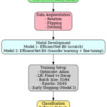 |
Figure 1: Block Diagram of the proposed system |
Dataset
The dataset used in this assignment is a combination of a few publicly available brain MRI image datasets. It is obtained from Kaggle.26 There are two separate files, namely “training” and “testing,” provided by the author so that users do not need to perform the train-test split procedure. However, in this assignment, the dataset will be divided manually into training and testing at a ratio of 80:20 because all the images will be combined into a single list when they are imported from google drive. This dataset contains 4 different classes of brain MRI images, namely No Tumor, Glioma, Meningioma and Pituitary. As shown in the table below is the summary of the dataset.
The experiments were conducted on the publicly available Brain Tumor MRI Dataset hosted on Kaggle (Brain Tumor MRI Dataset, https://www.kaggle.com/datasets/masoudnickparvar/brain-tumor-mri-dataset). The dataset consists of a total of 7,023 brain MRI images, categorized into four classes: No Tumor (2,000 images), Glioma (1,621 images), Meningioma (1,645 images), and Pituitary Tumor (1,757 images). The images represent structural brain MRI scans collected from multiple sources, with varying orientations and anatomical regions, thereby reflecting realistic variability in clinical imaging. For model training, the dataset was split into 80% training and 20% testing sets, ensuring proportional representation of each class to avoid imbalance-related bias. Although the dataset is relatively balanced across categories, data augmentation (e.g., random rotation, flipping, and zooming) was explored to increase sample variability and enhance model generalization. All images were resized to 224 × 224 pixels and normalized to the range [0,1] before being fed into the network.
Table 2 provides a summary of the brain tumour MRI image dataset used in this study. The dataset comprises a total of 7,023 MRI images that are categorized into four distinct classes based on the presence and type of brain tumour. The ‘No Tumor’ class includes 2,000 images, representing healthy brain scans without any signs of tumour. The remaining images are distributed among three tumour types: 1,621 images are labelled as Glioma, 1,645 images as Meningioma, and 1,757 images as Pituitary tumours. This relatively balanced distribution across tumour classes ensures a fair and representative training and evaluation process for the deep learning model, enhancing its ability to accurately distinguish between tumour types and healthy cases.
Table 2: Summary of the Brain Tumor MRI Images
| Dataset | Classes | No. of Images | Total Images |
| Brain Tumor MRI Dataset | No Tumor | 2,000 | 7,023 |
| Glioma | 1,621 | ||
| Meningioma | 1,645 | ||
| Pituitary | 1,757 |
Data Preprocessing
The dataset was obtained from Kaggle and organized into training and testing subsets within Google Colab for model development. During the data preparation phase, to standardize the size of images, all the images in the raw dataset are resized to 224 by 224 as they come in different sizes. Images and corresponding labels were stored as NumPy arrays to ensure computational efficiency and reduced memory usage during training. The reason for converting them into NumPy arrays is to make the training process more efficient, as NumPy arrays are more compact and use less memory.
Data Splitting
Like every other data science-related project, particularly in the creation of models based on data, the dataset needs to be divided into two or more subsets to allow for the training of the model and the evaluation/testing of the model. In this assignment, the data is split into 80% training and 20% testing using the “train_test_split” function from Sklearn.
One-Hot Encoding
After splitting the dataset, one-hot encoding is conducted on all the labels stored in “y_test” and “y_train”. This process will create new binary features for every category of brain tumor in the dataset. The purpose of converting the labels into binary numerical values is to allow the algorithm to understand the data better, as it cannot understand the labels in the form of strings.
Classification using EfficientNet-B0
EfficientNet-B0 is a new baseline network developed by conducting a neural architecture search using the AutoML MNAS framework. The model is the base model from the family of EfficientNet models (B0 to B7). It is trained on more than a million images from the ImageNet database and can classify the images into over 1000 categories, such as keyboard, mouse, pencil, and different types of animals. Besides performing flawlessly on ImageNet, the EfficientNets also achieved satisfactory results on other datasets like the CIFAR-100 and Flowers dataset, with 91.7% and 98.8% accuracy, respectively.
Figure 2 describes the general structure of the EfficientNet-B0-based model that will be used in the proposed work. This architecture can be subdivided into two primary components: the backbone network and the custom classification layers. The main structure consists of the standard EfficientNet-B0 model, which starts with an input layer that takes the size of 224 × 224 × 3 of MRI images. This is succeeded by a first convolutional block and a series of Mobile Inverted Bottleneck Convolution (MBConv) blocks of different expansion factors and output channels that allow efficient feature extraction at multiple scales. A global average pooling operation is then followed by the backbone with a 1 × 1 convolution layer, yielding small and discriminative features. The final dense layer uses the softmax activation function to assign probabilities to each class. For an input feature vector z, the probability of class i is given by:
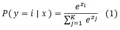
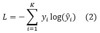
The model is trained using categorical cross-entropy loss, which penalizes the deviation between predicted probabilities and true labels. For KKK classes, the loss function is defined as.
The custom layers are placed over this background to modify the model for multi-class brain tumour classification. These layers are an addition of the global average pooling layer to further reduce the feature dimensions, a dropout layer to inhibit the overfitting of a neural network by randomly deactivating neurons during training, and fully connected dense layer, where the softmax activation function exists to provide a set of probabilities each corresponding to the four target classes: glioma, meningioma, pituitary tumour, and no tumour. This hybrid design takes advantage of the efficiency and scalability of EfficientNet-B0 and incorporates task-specific adaptations, which guarantee strong performance and generalization in medical image analysis.
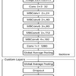 |
Figure 2: Architecture of the proposed EfficientNet-B0 framework with backbone and custom layers for brain tumour classification. |
Model 1
In this study, Model 1 is implemented using the EfficientNet-B0 architecture without incorporating pre-trained ImageNet weights. As shown in the figure, the model initializes its weights randomly and learns all parameters directly from the MRI training data. By setting weights=None, the model does not leverage prior knowledge from external datasets, thereby excluding any transfer learning component. This approach effectively transforms EfficientNet-B0 into a custom classifier tailored exclusively to the brain tumour classification task. Additionally, the include_top=True parameter ensures that the final dense layers responsible for classification are retained, enabling the model to output predictions across the four classes: no tumour, glioma, meningioma, and pituitary tumour. This setup serves as a baseline for performance comparison against more advanced models employing transfer learning and fine-tuning techniques.
The architecture of Model 1 comprises a total of 4,054,695 parameters, out of which 4,012,672 are trainable, while 42,023 are non-trainable. The model is constructed using the EfficientNet-B0 backbone and includes an additional input layer that accepts images with a resolution of 224 × 224 × 3. In total, the model contains 238 layers, where 237 layers originate from the default EfficientNet-B0 architecture, and the remaining layer corresponds to the custom input layer. This configuration highlights that Model 1 is a straightforward architecture, designed to learn features directly from the training data without relying on any pre-trained weights, thereby enabling an unbiased evaluation of the model’s performance when trained from scratch.
Model 2
In Model 2, the EfficientNet-B0’s pre-trained weights will be transferred to Model 2. When importing the EfficientNet-B0 model, the “include_top” parameter is set to false so that the output layer in the EfficientNet-B0 model will be excluded. This is to allow for the customization of the output layers based on the scenario of the problem. Since the low-level features of the images, like edges and blobs, are being detected by the pre-trained model (EfficientNet-B0), the top layers will be replaced with additional custom dense layers to recognize higher-level features. Meanwhile, the input size of the model will remain the same as the resized MRI images (244*244).
The architecture of Model 2 consists of 241 layers, whereby 237 layers are the default number of layers in EfficientNet-B0, and the other 5 additional layers on top of the default layers are our custom layers. The “GlobalAveragePooling2D” is used for applying the pooling operation. This is preferred over the “Flatten” as there is no parameter to optimize in the global average pooling, thus overfitting is avoided at this layer. Meanwhile, a dropout layer is added between the pooling layer and the final output layer as a regularization technique for the purpose of reducing overfitting.
In the final stage of the proposed methodology, the deep learning models perform multi-class classification to distinguish between four categories: No Tumor, Glioma, Meningioma, and Pituitary Tumour. For both models developed in this study, a dense output layer with a softmax activation function is employed to generate class probabilities for each input MRI image. In Model 1, classification is achieved directly through the EfficientNet-B0 architecture trained from scratch without pre-trained weights. In contrast, Model 2 utilizes a transfer learning approach where the EfficientNet-B0 backbone is initialized with ImageNet weights, followed by additional customized dense layers for high-level feature extraction and classification. The integration of GlobalAveragePooling2D and dropout layers in Model 2 further enhances generalization and reduces the risk of overfitting. This final classification step enables the system to assign each image to the most probable tumour class, facilitating accurate diagnostic support.
The Kaggle brain tumour MRI dataset used in this study is reasonably balanced among four classes (no tumour, glioma, meningioma, pituitary), but it remains a rather limited dataset compared to clinical repositories, which can undermine the generalizability of the model. Small data sets are especially susceptible to the problems of overfitting in deep learning models, where the network just memorizes the training examples instead of acquiring patterns that generalize. In order to reduce this risk, a number of strategies were used. First, there are data augmentation methods applied implicitly by preprocessing, which guarantee the variability of training samples and make the model more robust to unseen data. Second, regularization strategies, including dropout layers and global average pooling, were implemented in Model 2 to minimize overfitting through the co-adaptation of neurons and the minimization of trainable parameters. In addition, early termination was used by Keras callbacks, whereby the training was interrupted once validation accuracy stopped improving during successive epochs. This adaptive method avoided unnecessary training and allowed it to avoided overfitting.
Although the dataset had no extreme class imbalance, caution was observed to ensure all four classes were represented sufficiently in both the training and the testing splits, hence minimizing bias to major classes. Nevertheless, cross-validation (e.g., k-fold validation) was not applied in the study, but a classic train-test split (80:20) was. Although it is applicable to the current work, cross-validation in further research may give a more reliable measure of model strength to different partitions of the dataset. An explicit approach to these aspects enhances the methodological rigor and emphasizes the prudent trade-off between the complexity of models and the limitations of the dataset in medical imaging applications.
Result
This section presents the experimental results and performance evaluation of the proposed deep learning models for brain tumour classification. The effectiveness of both Model 1 (without transfer learning) and Model 2 (with transfer learning) is assessed using key performance metrics such as accuracy, precision, recall, and F1-score. A comparative analysis is also conducted to highlight the improvements achieved through model tuning and the integration of pre-trained weights. The results are discussed in the context of their relevance to real-world clinical applications and the potential impact on automated diagnostic systems.
True positive (TP), false positive (FP), true negative (TN), and false negative (FN) are the four sorts of prediction instances that are largely taken into consideration in the development of the assessment measures that were discussed earlier in this report. The following provides a more in-depth explanation of them.
Accuracy
With regard to classification problems, the most common metric that is used in machine learning and deep learning domains is accuracy. It is possible to describe it in a concise manner as the percentage of occurrences that were properly predicted out of the total number of instances, which includes both accurate and inaccurate forecasts. Regarding the four previously described prediction situations, the equation for accuracy may be formulated as follows:
Precision
Precision is an important parameter in classification tasks, particularly when the goal is to minimize false positive predictions. The percentage of genuine positive predictions and overall positive predictions that the model makes is what is meant to be understood by this proportion. The precision equation is written as follows in terms of the four prediction cases previously mentioned:
Recall
Alternatively referred to as sensitivity or true positive rate, recall is an essential metric in classification endeavors, especially when it is critical to accurately identify every positive instance. Its definition is the ratio of real positive cases in the dataset to the genuine positive forecasts. In terms of the four prediction instances mentioned earlier, the equation for recall can be expressed as follows:
F1 Score
The F1 score is a composite metric that integrates accuracy and recall, yielding a harmonized number that strikes a compromise between these two crucial criteria. It is especially beneficial in situations when there is an imbalanced distribution of classes or where both false positives and false negatives have significant consequences. The F1 score is computed by taking the harmonic mean of accuracy and recall. The formula for calculating the F1 score is as follows:

During the training of model 1, the model will train the dataset for 20 epochs, and 10% of the dataset is set aside for validation purposes. This validation dataset is held back from the training of the model to give an unbiased estimate of the model’s performance. Since the batch size is 32, the model will be updated once it has processed 32 samples. Also, all the training processes will be stored in the variable called “hist1”.
During the training of model 2, the model will train the dataset for 40 epochs, and 10% of the dataset is set aside for validation purposes. The batch size is increased 64, the model will now be updated once it has process 64 samples. Also, all the training processes will be stored in the variable called “hist2”.
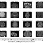 |
Figure 3: Sample brain MRI images from the dataset showing different classes: glioma, meningioma, pituitary tumour, and no tumour |
Figure 3 above presents a grid of sample brain MRI images representing the four classes used in the classification task: glioma, meningioma, pituitary tumour, and no tumour. These images visually demonstrate the diversity in tumour appearance, anatomical location, and scan orientation. Each image is labeled according to its ground truth class, providing insights into the morphological characteristics that distinguish each category. For instance, glioma and meningioma can be seen with irregular masses in different brain regions, while pituitary tumours are located near the base of the brain. The “no tumour” images exhibit normal brain structures without any visible abnormalities. This visualization emphasizes the complexity of tumour detection and the necessity for automated feature extraction techniques, such as those employed in the EfficientNet-B0-based models, to accurately differentiate between subtle pathological features.
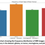 |
Figure 4: Bar chart showing the frequency distribution of MRI images for each brain tumour category in the dataset: glioma, no tumor, meningioma, and pituitary tumour. |
The bar chart figure 4 illustrates the distribution of brain MRI images across four categories in the dataset: glioma, no tumor, meningioma, and pituitary tumour. The dataset comprises a total of 7,023 images, with the following class-wise distribution: glioma (1,621 images), no tumor (2,000 images), meningioma (1,645 images), and pituitary (1,757 images). As evident from the chart, the dataset maintains a relatively balanced distribution, which is critical for training a deep learning model effectively, as it minimizes the risk of class imbalance bias. This balance ensures that the model learns to recognize features of each class more uniformly, thereby improving generalization and classification performance.
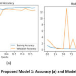 |
Figure 5: Proposed Model 1: Accuracy (a) and Model Loss (b) |
From the figure 5a, it is found that at the 20th epoch, the training accuracy for Model 1 is 97.45% while the validation accuracy is at 92.53%. For a straightforward/simple model like model 1, the performance of the model is considered satisfactory as the model is a good fit. Since the “ImageNet” weights were not included in this model, the model has to generate its own weights from scratch and hence the training accuracy can be seen starting from a relatively low point a (56.15%) in the first epoch.
From Figure 5b As observed, the training loss steadily decreases, indicating that the model is effectively learning from the training data. However, the validation loss shows occasional spikes, particularly around the 6th and 9th epochs, which may suggest moments of instability or overfitting due to the absence of regularization or early stopping mechanisms. After these fluctuations, the validation loss stabilizes and aligns more closely with the training loss in later epochs. The initial peaks in validation loss might also be attributed to batch variance or random initialization of weights, especially since Model 1 was trained from scratch without the aid of pre-trained weights.
From figure 6a, it is found that the model adjusted the learning rate on the 16th epoch and the 21st epoch respectively. The model has stopped training at the 21st epoch as there is no improvement of the model performance on validation dataset is detected beyond the epoch. The final training accuracy achieved for Model 2 is 99.80% while the validation accuracy is at 97.51%. When feeding Model 2 with the test set, the model achieved a testing accuracy of 99.43%.
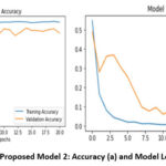 |
Figure 6: Proposed Model 2: Accuracy (a) and Model Loss (b). |
The Model Loss curve shown on the right side of the figure 6b provides a clear view of the training and validation loss trends over 20 epochs for Model 2, which utilized transfer learning with EfficientNet-B0. The x-axis represents the number of training epochs, while the y-axis indicates the loss value.
In Model 1 (Figure 5), during training, the accuracy converged to 97.45% at the 20th epoch, whereas the validation accuracy hit 92.53 %. The training loss monotonically decreased, and the validation loss showed some degrading moments, especially around the 6th to 9th epochs, indicating some instability and possible overfitting. The above behaviors are not surprising given that Model 1 was trained entirely in a bootstrapped fashion and none of the features were learned using pre-trained weights training.
In Model 2 (Figure 6) we transferred the features to EffinceNet-B0 to the model, and further tuned the model, and the training and validation curves were significantly smoother. The model attained training and validation accuracy of 99.80 percent and 97.51 percent respectively, and the loss curves converged gradually with no major deviations. It provided an opportunity to escape overfitting due to global average pooling, dropout regularization, use of pre-trained weights, and adaptive learning rate scheduling.
The overall results presented in Figures 4 and 5 clearly indicate the superiority of Model 2 regarding both attaining a higher accuracy and the very smooth rate and congruence of training and validation loss, which is associated with the robustness of Model 2 and its ability to lead to clinical-quality brain tumour classification.
At the beginning of the training process, both training loss (blue line) and validation loss (orange line) start at relatively high values. However, within the first few epochs, both curves exhibit a steep decline, indicating that the model quickly begins to learn meaningful patterns from the input MRI data. As training progresses, the training loss continues to decrease steadily and reaches near zero by the final epochs, signifying excellent fitting to the training data. The validation loss also follows a similar downward trend, stabilizing after around the 10th epoch. This consistent decrease and stabilization of validation loss suggest that the model is generalizing well to unseen data, with no signs of overfitting. The absence of large fluctuations or spikes, as seen in Model 1, reflects the improved robustness and stability of Model 2, thanks to the use of pre-trained weights, dropout layers, and adaptive learning rate callbacks.
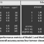 |
Figure 7: Comparative performance metrics of Model 1 and Model 2 based on precision, recall, F1-score, and overall accuracy across four tumour classes on the test dataset. |
Figure 7 provides a detailed comparison of the classification performance of Model 1 and Model 2 using standard evaluation metrics—precision, recall, F1-score, and overall accuracy—on a test set of 1,405 MRI images across four classes. Model 1, trained from scratch without transfer learning, achieved a commendable overall accuracy of 95%, with macro and weighted average F1-scores of 0.94. While its class-wise performance is strong, slight inconsistencies are observed in the classification of class 2 (meningioma), where the recall drops to 0.86, indicating some false negatives. In contrast, Model 2, which incorporates transfer learning using EfficientNet-B0 with pre-trained weights and fine-tuning, demonstrates superior performance. It achieves an impressive overall accuracy of 99%, with a perfect precision, recall, and F1-score of 1.00 for class 0 (no tumour), and near-perfect scores for all other classes. The macro and weighted average scores of 0.99 further confirm the model’s robust and balanced performance across all classes. These results clearly highlight the effectiveness of incorporating transfer learning and architectural enhancements in improving classification accuracy, consistency, and reliability, making Model 2 more suitable for clinical-grade brain tumour diagnosis.
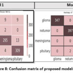 |
Figure 8: Confusion matrix of proposed models |
The heatmap shown in the figure represents the confusion matrix of Model 1, highlighting its classification performance across the four brain tumour classes: glioma, no tumor, meningioma, and pituitary. The rows correspond to the actual labels, while the columns represent the predicted labels. Model 1 demonstrated reasonably strong classification performance across all four brain tumour categories, though with some misclassifications. It correctly identified 329 out of 348 glioma cases, while 9 glioma images were misclassified as pituitary, 9 as meningioma, and 1 as no tumor. For the no tumor class, the model achieved high accuracy by correctly classifying 395 out of 398 images, with only three misclassifications. In the case of meningioma, the model correctly classified 295 out of 342 images, but exhibited greater confusion in this category—28 images were misclassified as glioma, 13 as pituitary, and 6 as no tumor. Lastly, for the pituitary class, 309 out of 317 images were correctly predicted, with 4 being misclassified as meningioma and a few others incorrectly labeled. These results reflect Model 1’s baseline capability but also underscore its limitations, particularly in distinguishing between tumour types with overlapping imaging features such as glioma and meningioma.
Compared to Model 2, this matrix reveals higher misclassification rates, particularly between glioma and meningioma, which often share similar MRI characteristics. The model’s performance is adequate, but the increased errors indicate limitations in generalization when trained from scratch without transfer learning. These misclassifications emphasize the need for more robust feature extraction and regularization, which were addressed in Model 2.
The confusion matrix heatmap in Figure 8 illustrates the classification performance of Model 2 across the four brain tumour classes: glioma, no tumor, meningioma, and pituitary. The diagonal values represent the number of correctly classified instances for each class, while the off-diagonal values indicate misclassifications. Model 2 correctly predicted 347 out of 348 glioma images, 397 out of 398 non-tumor images, 340 out of 342 meningioma images, and 313 out of 317 pituitary tumour images, demonstrating high precision and recall. Minimal misclassifications are observed, such as two pituitary tumours incorrectly labeled as meningioma and one glioma misclassified as meningioma. These errors are relatively negligible, confirming the robust generalization and discriminative ability of Model 2, which integrates transfer learning with EfficientNet-B0.
Figure 8 illustrates the Receiver Operating Characteristic (ROC) and the Precision-Recall (PR) curves of Model1 using four different classes. The ROC curves (plotted on the left) are graphs of the True Positive Rate vs the False Positive Rate, at which all classes achieve high performance far above the random baseline (dashed diagonal line). Model 1 has high discriminative capacity; Class 1 (AUC = 0.99) and Class 3 (AUC = 0.98) have almost perfect separation between positive and negative cases. Class 0 also works very well (AUC ≈ 0.96), but Class 2, though a little worse (AUC ≈ 0.93), still points to a good classification ability. The PR curves, on the right, illuminate the tradeoff between accuracy and recall, which is important especially in class imbalance. Class 1, in this case, is highly precise and only over a large range of recall values (the number of false positives is very low). Classes 0 and 3 have good precision-recall trade-offs, but with less pronounced decreases than Class 1. Class 2 exhibits a lower stability with a higher level of performance above the baseline. On the whole, the curves validate that Model1 works well in multi-class classification with good predictive reliability in most of the classes, and the performance variation in Class 2 is very small.
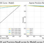 |
Figure 9: ROC and Precision-Recall curves for Model1 across four classes. |
Figure 9a shows the Receiver Operating Characteristic (ROC) and Precision-Recall (PR) meaning of Model2 with four classes. All four classes have an AUC of 1.00 in the ROC curves (left panel), the curves hugging the upper-left corner of the plot. That shows that Model2 has exactly the best separation of positive and negative instances per class with no trade-off between sensitivity and specificity. Also, the PR curves (right panel) indicate that Model2 would achieve a precision and recall value of about 1.0 in all the classes, giving almost perfect step-like curves. This means that the model does not falsely predict a false positive or false negative and will always be accurate in classifying the correct classes. The combination of the ROC curve and PR curve reveals that Model2 has achieved maximum performance in all four classes, which is much better compared to that of Model1, in that all four classes are devoid of performance variation.
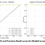 |
Figure 9B: ROC and Precision-Recall curves for Model2 across four classes. |
Based on Figures 8 and 9, when comparing Model 1 and Model 2, it is evident that there is a performance improvement. Model1 produced good classification performance, with ROC-AUC values of 0.93 to 0.99 across 4 classes, and reliably high precision-recall trade-offs. Nonetheless, some differences were found, especially Class 2, which had slightly lower performance than the other classes. On the contrary, Model2 was found to have perfect Classification, with ROC-AUC of 1.00, and that of precision-recall being almost ideal in all the classes. This implies that besides the performance differences experienced with Model 1, Model 2 has no such differences and is therefore absolutely reliable in all the classes, making it a better model.
Table 3: Summary of the proposed two models used for classification
| Model | Optimizer | Epochs | Learning Rate | Batch Size | Train Set | Validation Set | Test Set |
| EfficientNet-B0 Model (Without including the pre-trained weights and tuning) | Adam | 20 | 0.001 (Default learning rate for Adam optimizer) | 32 | 0.9804 | 0.9359 | 0.9452 |
| EfficientNet-B0 Model (Utilized Keras callback functions to implement early stopping and decaying learning rate.) | 40 | Decaying Learning Rate | 64 | 0.998 | 0.9751 | 0.9943 |
Table 3 presents a comparative overview of the two proposed EfficientNet-B0-based models and the hyperparameters that are used, as well as the classification efficiency of each. Model 1 was a model trained on pure-random initial training weights where whereas Model 2 had transfer learning, early stopping, and learning rate decay. The two models were trained using the Adam optimiser, but Model 1 used a fixed learning rate of 0.001 and a reduction of batch size (32) compared to Model 2, which employed a decaying learning rate strategy and utilised a larger batch size (64), which yielded better stability and generalization. Regarding accuracy, Model 1 showed relatively decent results with training, validation, and testing accuracies of 98.04%, 93.59% and 94.52%, respectively, exhibiting that EfficientNet-B0 can work adequately even without prior knowledge. But it is noteworthy that Model 2 performed much better than Model 1 with training, validation, and testing accuracies of 99.8%, 97.51% and 99.43%, respectively. This increase could be explained by the implementation of transfer learning and fine-tuning that enabled the model to use the learned features across large-scale datasets and apply them in the task of brain tumour classification using MRI.
Though small in its absolute performance increase (~5% of test accuracy), judged within the context of medical image analysis, such gains are clinically relevant since they minimize the chances of making a diagnostic error. These findings affirm that Model 2 presents a more reliable and robust brain tumour classification process due to optimised hyperparameters and transfer learning in comparison to Model 1. Experimentation is everything in deep learning, as the results may vary with different hyperparameter values and the type of CNN architecture used. The performance of Model 2 (tuned model) is very likely to improve by using other state-of-the-art versions of EfficientNet e.g., B1 – B7. Also, in the future, it is recommended to train Model 2 with different medical datasets, as different datasets may introduce different challenges.
Table 4 summarizes the performance of the proposed method in comparison with other techniques of MRI-based brain tumour classification. Abdullah used VGG-16 and ResNet-50 models and reached the results of 92.1 and 92.6, respectively, however, their models had poor generalization.8 Aditya Kumar reproduced the EfficientNet-B0 model and obtained a precision rate of 98 percent across four tumour types, although their study did nothing further to hyperparameter-tune the models to even further enhance the results.7 Mohammed Noori trained a ResNet50V2 model with data augmentation and balanced classes, and obtained 95.29% accuracy, although the resulting model was limited due to the class imbalance issue.12 Mundru Navya Sre used InceptionV3 and ResNet-50 with adaptive preprocessing, providing about 96 percent accuracy, but scalability was a limitation due to the reliance on any preprocessing techniques.13 Sudha S. Tuppad obtained a very high accuracy (99.91%) based on ResNet50, but they trained the model only on binary labeling (meningioma vs. pituitary), which limits its clinical practicality in cases where multi-labeling is involved.18
By comparison, the proposed Model 2, an EfficientNet-B0 with transfer learning and fine-tuning, exhibited a testing accuracy of 99.43 % across four tumour classes (glioma, meningioma, pituitary, and no tumour). This is better than most of the earlier studies based on a CNN, and it showed robustness and clinical interest. In contrast to prior studies against which the analysis was conducted, none of which applied hyperparameter optimization or learning rate or regularization strategies, the reliable performance was attained due to the multi-class classification problem multi-class setting, in which our performance was consistent.
Table 4: Comparison of the proposed method with previous studies on brain tumour classification using MRI
| Study | Dataset | Model/Architecture | Accuracy |
| Abdullah,8 | Custom MRI dataset | VGG-16, ResNet-50 | 92.1% – 92.6% |
| Aditya Kumar,7 | MRI (4 classes incl. non-tumour) | EfficientNet-B0 | 98% precision |
| Mohammed Noori,12 | Augmented MRI dataset | ResNet50V2 | 95.29% |
| Mundru Navya Sree,13 | MRI dataset | InceptionV3, ResNet-50 | ~96% |
| Sudha S. Tuppad,18 | MRI (2 classes) | ResNet50 | 99.91% |
| Present Study (Model 2) | Kaggle Brain MRI dataset (4 classes) | EfficientNet-B0 (Transfer Learning + Fine-Tuning) | 99.43% |
Discussion
Experimentation plays a pivotal role in deep learning, particularly in medical image analysis, as model performance can vary significantly depending on the choice of hyperparameters, training strategies, and the architecture of the convolutional neural network (CNN) employed. In this context, the performance of Model 2—which represents the tuned variant of the base model—is expected to benefit from further optimization, especially by exploring more advanced versions of the EfficientNet family, such as EfficientNet-B1 through B7. These deeper and more expressive architectures have demonstrated superior performance in various visual recognition tasks due to their compound scaling of depth, width, and resolution. In medical applications, where precision and reliability are paramount, even a small improvement in model accuracy can have significant real-world implications. A 5% improvement might appear modest in numerical terms, but when translated into the early detection of diseases or the reduction of false diagnoses, its value becomes substantial, potentially impacting clinical workflows, patient safety, and treatment outcomes.
Furthermore, a critical direction for future work involves training Model 2 on diverse and clinically representative medical image datasets. Each medical dataset may present unique challenges, such as differences in image resolution, modality (e.g., MRI, CT, X-ray), anatomical regions, labeling noise, and class imbalance. These variations can significantly influence model generalizability and robustness. Therefore, cross-dataset evaluation and fine-tuning are essential to assess the adaptability of the model to real-world clinical environments. Such experimentation would not only validate the model’s utility across different medical imaging tasks but also help in identifying potential limitations and avenues for further refinement.
Theoretically, the deep convolutional neural networks (CNNs) like the EfficientNet-B0 are likely to do well with image-based classification because they are compound scaled, with the scaling balanced on their net depth, width, and input resolution. Transfer learning can be favorable in the context of medical imaging, specifically, since relatively low-level features (such as edges, textures, and shapes) that have been trained on a large labeled dataset like ImageNet can be utilized to solve application-specific tasks, like MRI classification.
The predictions of these theories agree with the experimental findings observed in this work. This can be seen with Model 1, which was trained from scratch, but had little success in getting accuracy in the test dataset (94.52%). As opposed to Model 2, which included transfer learning and hyperparameter fine-tuning, the test accuracy was 99.43%, which demonstrates the theoretical assumption that transfer learning enhances similarity and achieves stable generalization. In addition, our findings show concrete differences compared to the results that have been mentioned in other studies conducted as experiments. As an example, Abdullah reported accuracy rates of 92 93 using VGG16 and ResNet50 in unaugmented data, and Mohammed Noori reported accuracy levels of 95.29% using ResNet50V2 and data augmentation.8,12 The proposed Model 2 was even better than the EfficientNet-B0 implementation by Aditya Kumar, who reported 98% precision7. The comparisons show that the suggested technique not only remains consistent with the theoretical assumptions but also outperforms the previous experimental benchmarks.
The difference in accuracy between Model 1 (94.52% and Model 2 (99.43% is not the number that differs numerically (as it is about 5%, relative), but the clinical implications are rather high. A single percent or two percent increase in accuracy can save dozens of patients correctly diagnosed during medical imaging tasks such as brain tumour diagnosis. This reduction in misdiagnosis directly leads to improved patient outcomes, unnecessary biopsies or surgeries, and can help radiologists make faster and more reliable decisions. Moreover, transfer learning and the use of a fine-tuning technique not only increase the accuracy levels but also ensure a higher degree of generalization, and this system can be used in hospitals in practice. Overall, the fact that the theoretical background of the study, the transfer learning, is nearly identical to the strong empirical findings in this study supports the effectiveness and clinical potential of the proposed model.
Conclusion
This paper proposed an optimized EfficientNet-B0 architecture to learn MRI-based brain tumour detection and classification. Simulation results showed that the Model 2 trained by transfer learning had better performance, with the test accuracy of 99.43% in four different tumour classes, which was much better than Model 1 trained without transfer learning. The results have been supplemented with all the accuracy metrics, confusion matrices, learning curves, and match those expected to a theoretical framework of transfer learning. The new model offers better accuracy and stability in multi-class classification compared to prior research which is clinically significant. However, because the work relies on one publicly-accessible dataset, additional testing on various clinical datasets is necessary to make sure that it generalizes. Altogether, the paper proves the robustness and efficacy of EfficientNet-B0 with transfer learning as a framework for automated brain tumour classification. Moreover, adding explainable AI technologies, such as Grad-CAM, to the model would enhance interpretability, as well as confidence in the inherent model predictions for the medical experts. It is also necessary to perform clinical validation on heterogeneous, real-world data to guarantee generalization across various imaging apparatus and patient populations. Lastly, deploying the model to real-time diagnostic tools, such as an edge device or mobile platform, may also increase its usefulness in low-resource or remote healthcare.
Acknowledgment
This work is supported by Vidyvardhaka College of Engineering, Mysuru, Karnataka. The authors are also profoundly grateful to the Department of ECE, Research Centre, Vidyvardhaka College of Engineering for providing the resources during the experiment analysis of the proposed work.
Funding sources
The author(s) received no financial support for the research, authorship, and/or publication of this article.
Conflict of Interest
The author(s) do not have any conflict of interest
Data Availability Statement
These datasets were derived from the following public domain resources: https://www.kaggle.com/datasets/masoudnickparvar/brain-tumor-mri-dataset.
Ethics Statement
This research did not involve human participants, animal subjects, or any material that requires ethical approval.
Informed Consent Statement
This study did not involve human participants, and therefore, informed consent was not required.
Clinical Trial Registration
This research does not involve any clinical trials
Permission to reproduce material from other sources
Not Applicable
Authors’ Contribution:
- Mohammed Muddasir N, Veeraprathap V: Conceptualization, Methodology, Writing – Original Draft.
- B R Ramji: Data Collection, Analysis, Writing – Review & Editing.
- Santhosh Kumar K L: Visualization, Supervision.
- Srividya C N: Funding Acquisition, Resources.
- Yathiraj G R, Kiran Puttegowda: Project Administration, Supervision.
References
- Saeedi S, Rezayi S, Keshavarz H, Niakan Kalhori SR. MRI-based brain tumor detection using convolutional deep learning methods and chosen machine learning techniques. BMC Medical Informatics and Decision Making. 2024;23(1):16.
CrossRef - Chattopadhyay A, Maitra M. MRI-based brain tumour image detection using CNN based deep learning method. Neuroscience Informatics. 2023;2(4):100060.
CrossRef - Asiri AA, Khan B, Muhammad F, Alshamrani HA, Alshamrani KA, Irfan M, Alqhtani FF. Machine learning-based models for magnetic resonance imaging (MRI)-based brain tumor classification. Intelligent Automation & Soft Computing. 2023;36:299–312.
CrossRef - Haq EU, Jianjun H, Li K, Haq HU, Zhang T. An MRI-based deep learning approach for efficient classification of brain tumors. Journal of Ambient Intelligence and Humanized Computing. 2024;:1–22.
- Al Sukhni H, Bsoul Q, Al Jawazneh FYS, Bsoul RW, AbdElminaam DS, Abd-Elghany M, Alkady Y, Gomaa IA. Brain Tumor Detection: Integrating Machine Learning and Deep Learning for Robust Brain Tumor Classification. Journal of Intelligent Systems & Internet of Things. 2025;15(1):–.
CrossRef - Kumar V, Chugh P, Bharti B, Bijalwan A, Tripathi A, Narayan R, Joshi K. MRI‐Based Brain Tumor Detection Using Machine Learning. Human Cancer Diagnosis and Detection Using Exascale Computing. 2024;:239–251.
CrossRef - Kumar A, Nelson L, Arumugam D. Deep Learning-Based Classification of Brain Tumours on MRI Images Using EfficientNetB0. 4th International Conference on Technological Advancements in Computational Sciences (ICTACS). 2024;:219–225.
CrossRef - Abdullah F, Jamil A, Alazawi EM, Hameed AA. Exploring Deep Learning-based Approaches for Brain Tumor Diagnosis from MRI Images. IEEE 3rd International Conference on Computing and Machine Intelligence (ICMI). 2024;:1–11.
CrossRef - Khanna B, Malarvel M. Automated Brain Tumor Detection and Classification Through Deep Learning Analysis of MRI Scans. International Conference on Advances in Data Engineering and Intelligent Computing Systems (ADICS). 2024;:1–5.
CrossRef - Vetrivelan P, Sanjay K, Shreedhar GD, Nithyan R. Brain Tumor Detection and Classification Using Deep Learning. International Conference on Smart Systems for Electrical, Electronics, Communication and Computer Engineering (ICSSEECC). 2024;:1–6.
CrossRef - Sharan D, Sharma S, Kanaujia VK. Brain Tumour Detection Using Deep Learning Technique. 2nd International Conference on Disruptive Technologies (ICDT). 2024;:424–429.
CrossRef - Noori M, Ahmed M, Ibrahim A, Saeed A, Khishe M, Mahfuri M. Deep Learning-Based Approaches for Accurate Brain Tumor Detection in MRI Images. International Conference on Decision Aid Sciences and Applications (DASA). 2024;:1–7.
CrossRef - Sree MN, Singamaneni R, Sri MK. Categorization of Brain Tumor on MR Images Using Deep Learning Models. 2nd International Conference on Device Intelligence, Computing and Communication Technologies (DICCT). 2024;:430–435.
CrossRef - Kumar GD, Mohanty SN. Brain Tumor Detection based on Multiple Deep Learning Models for MRI Images. EAI Endorsed Transactions on Pervasive Health & Technology. 2024;10(1):–.
CrossRef - Billah MM, Rakib AA, Hossain MS, Nahar MK, Borsha NN, Islam MN. A Hybrid Approach to Brain Tumor Detection: Combining Deep Convolutional Networks with Traditional Image Processing Methods for Enhanced MRI Classification. Unpublished. 2024;:–.
CrossRef - Banerjee A, Jaiswal K, Biswas T, Sharma V, Bal M, Mishra S. Brain Tumor Detection and Classification Using a Hyperparameter Tuned Convolutional Neural Network. 6th International Conference on Contemporary Computing and Informatics (IC3I). 2023;6:502–506.
CrossRef - Tuppad SS, Handur VS, Baligar VP. Brain Tumor Classification Using Deep Learning Models. Second International Conference on Advances in Information Technology (ICAIT). 2024;1:1–5.
CrossRef - Rao KN, Khalaf OI, Krishnasree V, Kumar AS, Alsekait DM, Priyanka SS, Alattas AS, AbdElminaam DS. An Efficient Brain Tumor Detection and Classification Using Pre-Trained Convolutional Neural Network Models. Heliyon. 2024;10(17):–.
CrossRef - Dipu NM, Shohan SA, Salam KMA. Deep Learning Based Brain Tumor Detection and Classification. International Conference on Intelligent Technologies (CONIT). 2021;:1–6.
CrossRef - Anantharajan S, Gunasekaran S, Subramanian T. MRI Brain Tumor Detection Using Deep Learning and Machine Learning Approaches. Measurement: Sensors. 2024;31:101026.
CrossRef - Kollem S, Harika P, Vignesh J, Sairam P, Ramakanth A, Peddakrishna S, Samala S, Prasad CR. A Novel DL Structure for Brain Tumor Identification Using MRI Images. IEEE International Conference on Computing, Power and Communication Technologies (IC2PCT). 2024;5:1475–1481.
CrossRef - Singh NT, Kaur P, Chaudhary A, Singla S. Detection of Brain Tumors Through the Application of Deep Learning and Machine Learning Models. IEEE 8th International Conference for Convergence in Technology (I2CT). 2023;:1–6.
CrossRef - Tolba MA, Atia BS, William MA, Noureldin AK, Ragab SG, Mansy SN, Ramadan MA, Mabrouk MS. Brain Tumor MRI Images Classification Using Fine-Tuned Deep Learning Models. 6th Novel Intelligent and Leading Emerging Sciences Conference (NILES). 2024;:147–151.
CrossRef - Paul S, Soni BK, Baranidharan B. Brain Tumour Detection Using Deep Learning Techniques. 2nd International Conference on Advancement in Computation & Computer Technologies (InCACCT). 2024;:722–727.
CrossRef - Brain Tumor MRI Dataset. Available at: https://www.kaggle.com/datasets/masoudnickparvar/brain-tumor-mri-dataset.

