
Manuscript accepted on :24-09-2025
Published online on: 20-10-2025
Plagiarism Check: Yes
Reviewed by: Dr. Ramdas Bhat
Second Review by: Dr. Samina Akram
Final Approval by: Dr. Kamal Upreti
Tulip Das1,3 , Chinmaya Kumar Nayak2 and Parthasarathi Pattnayak3*
1Faculty of Engineering and Technology, SRI SRI University, Cuttack, India.
2School of Computer Applications, KIIT Deemed to be University, Bhubaneswar, India.
Corresponding Author E-mail: parthakiit19@gmail.com
Abstract
Alzheimer's disease (AD), also called dementia, is a neurological illness that progressively impairs memory and cognitive functioning. It hinders critical mental processes like reasoning, memory, and judgement. While precise diagnosis is often achieved through the use of standard imaging techniques such as CT, MRI, and PET, deep learning (DL) frameworks provide a quicker, less technologically demanding, and less human intervention method. These models, which have been validated by clinically collected medical data, also become more accurate with time and can help predict AD. This paper presents a model built on AI that consists of two main stages: a voting classifier that uses transfer learning (TL) and machine learning (ML) based on permutations. In the first stage of the model, DenseNet-121 and DenseNet-201 are used for feature extraction. In the second stage, three distinct machine learning classifiers are employed for classification: Naïve Bayes, Support Vector Machine (SVM) and XG Boost. To test the model, 6,400 photos from Kaggle's training dataset were used. The results show that this suggested model works better than current cutting-edge methods. Based on these results, the model may be used to create clinically useful techniques for AD diagnosis using MRI images.
Keywords
Alzheimer’s Disease; DenseNet-121; DenseNet-201; Gaussian Naïve Base; SVM; XG Boost
| Copy the following to cite this article: Das T, Nayak C. K, Pattnayak P. Enhanced Hybrid AI-Based Framework for Improving the Detection and Diagnosis of Alzheimer’s Disease. Biomed Pharmacol J 2025;18(October Spl Edition). |
| Copy the following to cite this URL: Das T, Nayak C. K, Pattnayak P. Enhanced Hybrid AI-Based Framework for Improving the Detection and Diagnosis of Alzheimer’s Disease. Biomed Pharmacol J 2025;18(October Spl Edition). Available from: https://bit.ly/47wXXMJ |
Introduction
AD is a neurological illness that leads to destruction of brain cells, which gradually deteriorates memory and impairs fundamental cognitive capacities. Changes in the brain are indicative of this disease, which ultimately leads to the loss of neurons and their connections. The WHO estimates that 10 million new instances of AD are diagnosed each year, and that around 50 million individuals suffer from dementia. After age 85, the chance of having AD eventually rises to 50%. AD ultimately results in death by destroying the area of the brain responsible for breathing and heart monitoring.1,2,3 There are three phases of AD: extremely mild, medium, and moderate.4,5 The middle stage of degeneration eventually makes it difficult for patients to be independent, making it difficult for them to do many of the most basic daily duties. Speech problems stem from incorrect word substitutions brought on by a memory loss. Additionally, fewer people are able to read and write.6,7,8,9 The risk of failing increases as AD advances due to a decline in the coordination of complex motor processes. By this stage, the individual may experience a decline in their ability to identify immediate relatives and their cognitive impairments intensify.10,11 Problems arise when long-term memory is disrupted. However, AD can also be aided by aging itself, as well as a variety of health, environmental and lifestyle factors.12,13,17,18 They include heart issues, social isolation and inadequate sleep all of which increase the risk of AD.
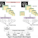 |
Figure 1: Proposed Model’s Block Diagram. |
From the study, the following contributions may be deduced:
An AD detection method was developed using a hybrid technique that combines permutation-based ML and TL. Three hybrid DenseNet-121 models were employed to emulate the detection of AD using SVM, GNB and XGB ML classifiers in different combinations. The hybrid Des-neNet-121
SVM model gave better results was opted for more simulation.19,20
DenseNet-121 and DenseNet-201, which are both based on transfer learning (TL), were used to extract features in practical applications.
Ultimately, three of the most widely employed ML classifiers for classification—SVM, Gaussian Naive Bayes (GNB), and XG Boost (XGB)—were sequentially developed.
A voting classifier based on permutations was employed the final accuracy observation.
For evaluation, 1000 epochs and the Adam optimizer were used to implement the suggested model.16,21,23,24,25
Literature Review
In this study, Bin.c (binary classification) of AD was primarily focused and their suggested model which was not flexible was developed using a smaller dataset. A larger dataset has been used for training for several of these writers. They had carried out binary classification. Past models are compared in the table below.
To execute the models, in table 1 smaller datasets from have been used. Nevertheless, suggested model does not use binary classification and was tested on a sizable dataset. Alternatively, it categorizes Alzheimer’s into four groups: Very mild, mild, moderate, and non- demented.
Table 1: Comparison of Existing Models.
| Study | Method | Purpose | Drawbacks |
| [6] | VGG16, 2D-CNN | To use ensemble-based CNN for AD classification. | The dataset included 798 T1-weighted image scans, with an accuracy of 90.36% and Bin.c performance. to apply 2D-CNN to separate AD from MCI pictures. |
| [9] | CNN, SVM, k-NN | To apply SVM and k-NN to identify MCI from AD. | The dataset included 1311 weighted image scans from T1 and T2, which were processed using Bin.c with a 75% accuracy rate. To use SVM-CNN and KNN to separate AD from MCI pictures. |
| [10] | FNN, DTCWT, PCA | To create a CAD system for the purpose of early AD diagnosis. | The dataset comprised 416 T1-weighted image scans, which were processed using Bin.c with a 90.06% accuracy rate. For swarm optimization, many feature reduction techniques as ICA, LDA, and PCA were applied. |
| [11] | CNN, SVM | Use a classifier based on SVM with a linear kernel to distinguish both AD and MCI. | With 69.37% accuracy, the dataset, which included 1167 T1-weighted imaging scans, executed Bin.c. utilizing SVM-CNN to separate AD from MCI images. |
| [14] | CNN, Data Augmentation | Using Cross-Modal Transfer Learning to Classify AD | By using Bin.c, the dataset consisting of 416 sMRI image scans achieved a successful accuracy percentage of 84%. |
| [15] | CNN, SVM | To use semi-supervised SVM-CNN to distinguish AD from MCI. | The dataset comprised 359 T1-weighted images, achieving an accuracy of 82.91% and performing better than Bin.c. In semi-supervised SVM, brain MRI images are differentiated. |
| [19] | CNN, SVM-REF | To use SVM-REF-CNN for AD classification. | 1167 T1-weighted image scans made up the dataset; it executed Bin.c with an accuracy of 81%. to use SVM-REF to differentiate between images of brain. |
| [22] | VGGNet16, VGGNet 19, ResNet18, ResNet50, ResNet 101, SqueezeNet, AlexNet, GoogleNet, Inceptionv3 | To use D.L. approaches for MRI images to identify AD. | There were 177 pictures in the dataset. The system achieved 84.38% accuracy while executing Bin.c. It may also be enhanced to include more neuroimaging techniques like PET scans as well as system features that include different aspects of AD. |
Materials and Methods
The DenseNet Model serves the purpose of amalgamating various machine learning classification techniques to derive feature maps from an image dataset employing a transfer learning approach. The ML classifiers are subsequently employed to categorize the feature map into four groups. Feature maps are extracted using Densenet121 and DenseNet201 models. Classification is performed using three distinct types of classifiers: Gaussian NB, SVM and XG Boost. The 6200 AD photo dataset from Kaggle is used by the suggested model. Figure 1 illustrates the several layers that make up the framework. Below is an explanation of the many building components of the suggested model. Using TensorFlow and the Python Keras package the model operates on a backend.
Source Dataset
6400 AD photos in all were gathered from the Kaggle database and utilized as the study’s database. It consists of 2240 VMD, 896 MD, 64 Mod D and 3200 ND, and grayscale photos with size of (208 × 176 × 3) pixels. Eighty percent of the evaluation dataset was used for training, while the remaining twenty percent was used for testing. The quantity of photos utilized for training and validation is displayed in Table 2. Figure.2. displays the instances of the images for each category.
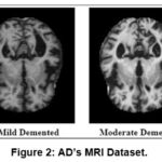 |
Figure 2: AD’s MRI Dataset. |
Table 2: Kaggle’s AD Dataset.
| Source Dataset | Class | Images for Training | Images for Validation | Total |
| Kaggle | Very Mild | 1792 | 448 | 2240 |
| Mild | 717 | 179 | 896 | |
| Moderate | 52 | 12 | 64 | |
| Non-Demented | 2560 | 640 | 3200 |
Preprocessing of Data
Normalization of Data
The updated Inception model maintains its numerical stability, thanks to data normalization. MRI pictures were essentially taken in grayscale. The normalization method was employed to expedite the training of MRI datasets in the proposed model.
Data Augmentation
A huge dataset is required to improve the model’s utility. Nevertheless, problems with obtaining these statistics include privacy and data constraints, in addition to a large number of websites. A variety of dataset augmentation techniques were used to address these issues. The initial quantity of data was greatly increased by these augmentation techniques. Methods including flipping an image horizontally, vertically, rotating it anticlockwise at 90, rotating it at 270, and brightening it by a factor of 0.7 are used. Figure 3 displays these five data augmentation techniques.
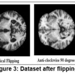 |
Figure 3: Dataset after flipping. |
The number of photos both before and after data augmentation is shown in Table 3. In addition, the quantity of photos in each class is uneven. The aforementioned procedures were followed in an effort to reduce this disparity. Following the implementation of these techniques, 10,760 photos were added to the original dataset. The quantity of recently updated photos is indicated in Table 3. It was only on the training photos that the augmentation was implemented. Previously, 2240, 896, 64 and 3200 were the training pictures for VMD, MD, Mod D and ND respectively. Following the augmentation, the count of training photos was 10,760 is displayed in table 3.
Table 3: Augmented AD Dataset.
| Class Name | Very Mild | Mild | Moderate | Non-Demented |
| Pre-Augmentation Images | 2240 | 896 | 64 | 3200 |
| Post-Augmentation Images (training) | 4800 | 2150 | 512 | 2800 |
| Post-Augmentation Images (testing) | 1098 | 538 | 128 | 700 |
Different DenseNet TL Models for Feature Extraction
DenseNet-121 and DenseNet-201 are applied to input images with 208 * 176 dimensions in the suggested model in order to extract feature maps. Table 4 displays the five convolutional blocks that make up the DesneNet121 model. The image is resized to match the dimensions of 112*112 of Conv-1 (first convolutional block). It then proceeds to the max pooling block, followed by Conv-2, resulting in a size of 56*56. Subsequently, it is forwarded to Conv-3, which yields a form of 28*28. It is then passed on to Conv-4, resulting in a shape of 14*14. Finally, it is delivered to Conv-5 resulting in a shape of 7*7. Conv-5 is first applied to the retrieved features, then the layer that performs global average pooling and lastly the dense layer which generates the output. DenseNet201 and DenseNet121 differ in how many convolution layers are employed in each con-volution block. DenseNet121 has 1024 filters in its last dense layer, while DenseNet201 uses 1920 filters as shown in table 5.
DenseNet-121 Model Based Feature Extraction
Following each dense block, Table 6 displays the filter visualization pictures for each convolution layer of DenseNet 121. The model suggested contains five convolutional blocks the images and single kernel and filters are displayed after each convolution layer in Table 6.
Table 4: Description of DenseNet 121’s Layers in a CNN.
| Convolutional Block | Con1 | Con 2 | Con 3 | Con 4 | Con 5 | |
| Convolutional Layers | Con 1- Con 1 | Con 1-1: Con 2-6 | Con 3-1: Con 3-12 | Con 4-1: Con 4-48 | Con 5-1: Con 5-32 | |
| Dimensions | I/p | 224*224 | 112*112 | 56*56 | 28*28 | 14*14 |
| O/p | 112*112 | 56*56 | 28*28 | 14*14 | 7*7 | |
| Filter | 7*7 | 1*1 | 1*1 | 1*1 | 1*1 | |
| Total | Filter | 64 | 128 | 512 | 896 | 1920 |
| Block Run | 1 | 6 | 12 | 48 | 32 | |
DenseNet-201 Model Based Feature Extraction
Table 7 presents the filter visualization picture of each DenseNet 201 convolution layer in addition to the processed images of each class after each dense block. In the suggested model, there are five convolutional blocks altogether. Table 7 displays the single kernel or filters and the pictures that follow each convolution layer.
Table 5: Explanation of CNN 201.
| Convolutional Block | Con 1 | Con 2 | Con 3 | Con 4 | Con 5 | |
| Convolutional Layers | Con 1- Con 1 | Con 2-1: Con 2-12 | Con 3-1: Con 2-24 | Con 4-1: Con 4-96 | Con 5-1: Con 5-64 | |
| Dimensions | I/p | 224*224 | 112*112 | 56*56 | 28*28 | 14*14 |
| O/p | 112*112 | 56*56 | 28*28 | 14*14 | 7*7 | |
| Filter | 7*7 | 1*1 | 1*1 | 1*1 | 1*1 | |
| Total | Filter | 64 | 128 | 512 | 896 | 1920 |
| Block Run | 1 | 6 | 12 | 48 | 32 | |
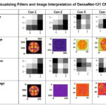 |
Table 6: Visualizing Filters and Image Interpretation of DenseNet-121 CNN Layers. |
Classification Through CNN-Hybrid ML
SVM, XG Boost, and Gaussian NB are the machine learning classifiers that receive the extracted features that were acquired from Block-5 of both DenseNet designs. Subsequently, these are conveyed to a compact layer to obtain an output. Table 8 and 9 illustrates the primary difference between the two models in their layer description by the frequency of block execution and the number of filters used at each layer.
Classifier: Gaussian NB
These are Bayesian-based supervised ML classification algorithms. They are useful in the computation of conditional probability. In these classifiers, each feature’s value is entirely independent. The values of any other feature have no bearing on these features. This classifier makes use of continuous data, which typically take continuous values related to the class in which they belong. Equation 1 provides the probable feature.
![]()
where v is a random observation value, σ2n is the Bessel corrected variance, μn is the mean of the values z linked to the class Cn.
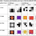 |
Table 7: Visualizing and illustrating each layer of the DenseNet-201 CNN. |
lassification Algorithm
XG Boost: Extreme Gradient Boosting, also known as XG Boost, is a highly optimized distributed gradient boosting framework renowned for its versatility, streamlined architecture, and efficiency. Along with other CNN models, this classifier is on larger unstructured datasets. The value of XGB is given in equation (2).
![]()
Where fm (z) defines the model update and the input training dataset (z) by less proficient learners from m to M.
Classifier SVM
With this method, every data point is treated as an n-dimensional space, and each feature value is treated as a coordinate value. After that, that designated classes are separated to produce the hyper-plane. Formula (3) yields the SVM classifier.
![]()
where the normal vector to the hyperplane is denoted as w. The expression wxzib indicates the ith output. b represents the overall input points. The term one is used to indicate a hard margin classifier for classifiable input data. zi is the kth dimensional real vector.
Table 8: Layers Description of DensNet-121.
| Block | Con -5 | Con-5 | Dense-4 | |
| Layers | Con-5-1: Con-5-32 | ML Classifiers | Dense | |
| Dimensions | Input | 14*14 | 7*7 | 4*4 |
| Output | 7*7 | 4*1 | 4*1 | |
| Filter | 1*1 | 1*1 | NA | |
| Total | Filter | 1024 | 1024 | NA |
| Block Run | 32 | 32 | 1 | |
Table 9: Hybrid DenseNet201 Model Layers’ Description.
| Block | Con-5 | Con-5 | Dense-4 | |
| Layers | Con-5-1: Con-5-64 | ML Classifiers | Dense | |
| Dimensions | Input | 14*14 | 7*7 | 4*1 |
| Output | 7*7 | 4*1 | 4*1 | |
| Filter | 1*1 | 1*1 | NA | |
| Total | Filter | 1920 | 1920 | NA |
| Block Run | 64 | 64 | 1 | |
Results
Hybrid DenseNet-201 Model Analysis
Three distinct ML classifiers are used to classify the retrieved features from DenseNet-121 models: SVM, GNB, NB and XG Boost. Data on train and validation loss as well as confusion matrix settings are used to assess the performance of these three models.
Losses in Training and Validation for Hybrid DenseNet-121 Models with different epochs
Figure 4 depicts the hinge loss, which shows variations in loss that occur throughout the model training. The hybrid models, DenseNet-121-SVM and hybrid DenseNet-121- Gaussian NB (Figure.4 (a) & (b)), achieved the lowest hinge loss during validation, whereas the hybrid DenseNet-121-XG Boost (Figure.4(c)) exhibits a greater hinge loss. Table 10 shows the computational features of combination DenseNet-121 models at different epochs, with a focus on hybrid DenseNet-121-SVM efficiency at the 1000th epoch. The training loss for DenseNet-121 with SVM at the 1000th epoch is 0.051 while the validation loss is 0.313.
Table 10: Hybrid DenseNet-121’s training and validation loss with a fixed batch size of 64 with different epochs.
| Epoch | 200 | 400 | 600 | 800 | 1000 | |
| SVM | Train | .264 | .14 | .089 | .068 | .051 |
| Valid | .554 | .467 | .422 | .394 | .313 | |
| GNB | Train | .265 | .141 | .88 | .065 | .051 |
| Valid | .497 | .402 | .348 | .323 | .33 | |
| XGB | Train | .262 | .125 | .86 | .059 | .05 |
| Valid | .531 | .45 | .405 | .384 | .372 | |
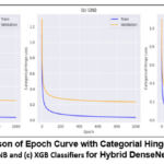 |
Figure 4: Comparison of Epoch Curve with Categorial Hinge Loss with (a) SVM, (b) GNB and (c) XGB Classifiers for Hybrid DenseNet-12. |
Comparison of Confusion Matrix for Hybrid DenseNet-121 Models
In Figure.5, the hybrid DenseNet-121 models with ML classifiers’ confusion matrix are displayed. These matrices illustrate both correct and incorrect predictions. Using the class names Mild, Very Mild, Moderate and Non-Demented each column is distinguished from the others. Diagonal values may be used to discover exactly how many images are categorized by a given model. The accuracy of all the DL models with DenseNet-121 using SVM outperforming other DL models with ML classifiers in terms of performance are illustrated in figure.6.
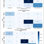 |
Figure 5: Hybrid DenseNet -121’s Confusion Matrix with ML Classifiers. |
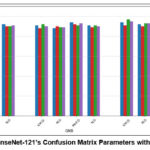 |
Figure 6: Hybrid DenseNet-121’s Confusion Matrix Parameters with the ML Classifiers. |
Table 11 exhibits the values of average precision (P), average specificity and sensitivity (Sp and S) average accuracy and average F1- score (F1) 64 is the batch size used to calculate these average parameters. It is evident that DenseNet-121-SVM produces testing results that are more consistent and superior.
Table 11: Hybrid DenseNet-121 Model’s Confusion Matrix Parameters (%).
| Type | Average | Accuracy | |
| SVM | F1 | 90 | 89.89 |
| SP | 96 | ||
| P | 92 | ||
| S | 89 | ||
| GNB | F1 | 89 | 89.18 |
| SP | 96 | ||
| P | 88 | ||
| S | 89 | ||
| XGB | F1 | 85 | 88.25 |
| SP | 95 | ||
| P | 90 | ||
| S | 83 |
Hybrid DenseNet-201 Model Analysis
Three distinct ML classifiers are used to classify the features retrieved from the DenseNet-201 model: Gaussian NB, SVM and XG Boost. These hybrid DenseNet-201 models’ performance are examined utilized confusion matrix settings and loss and validation data.
Hybrid DenseNet-201 Models: Training and Validation Losses with different epochs
Figure. 7 depicts hinge loss, which quantifies the variations in loss during the training of the model. SVM and GNB in Figure. 7 demonstrates the DenseNet-201 SVM and DenseNet-201 GNB achieves a loss. However, XGB in Figure 7 reveals that the validation hinge loos of DenseNet-201 XGB is higher than the other two hybrid models. Table 12 demonstrates that the hybrid DenseNet-201 GNB outperform the other three DL models. The training and validation loss of DenseNet-201 with GNB is 0.028 and 0.265 respectively.
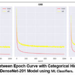 |
Figure 7: Comparison between Epoch Curve with Categorical Hinge Loss for the Hybrid DenseNet-201 Model using ML Classifiers. |
Table 12: Hybrid DenseNet-201 model with variable epochs and a fixed batch 64 experienced training and validation loss.
| Epoch | 200 | 400 | 600 | 800 | 1000 | |
| SVM | Train | .16 | .075 | .047 | .035 | .027 |
| Valid | .418 | .326 | .294 | .292 | .291 | |
| GNB | Train | .158 | .73 | .47 | .033 | .028 |
| Valid | .427 | .348 | .317 | .299 | .265 | |
| XGB | Train | .157 | .07 | .46 | .031 | .25 |
| Valid | .459 | .373 | .353 | .326 | .318 | |
Comparison of Confusion Matrix for Hybrid DenseNet-201 Model
Figure 9 displays the confusion matrices of the DenseNet-201 model using ML classifiers with a 64-batch size. These matrices show predictions that are accurate as well as inaccurate of all DL models’ accuracy while using ML classifiers as in figure 10. With ML classifiers, Gaussian NB outperforms the other DL models. The average of precision, sensitivity, sensitivity, F1-score accuracy and performance comparison of all DenseNet-201 hybrid models are shown table 13. With batch size 64, these average parameters are found. It is evident that using DenseNet-201-Gaussian NB leads to more consistent and improved testing performance.
Table 13: DenseNet-201 Confusion Matrix Parameters (%).
| Type | Average | Accuracy | |
| SVM | F1 | 92 | 91.03 |
| SP | 96 | ||
| S | 92 | ||
| P | 93 | ||
| GNB | F1 | 90 | 91.75 |
| SP | 97 | ||
| S | 89 | ||
| P | 93 | ||
| XGB | F1 | 92 | 91.13 |
| SP | 98 | ||
| S | 92 | ||
| P | 93 |
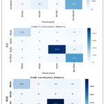 |
Figure 8: DenseNet-201’ Confusion Matrix with the ML Classifiers. |
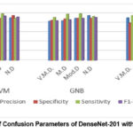 |
Figure 9: The Matrix of Confusion Parameters of DenseNet-201 with Three ML Classifiers. |
Discussion
DenseNet-201-GNB Classifier vs Hybrid DenseNet-121-SVM Comparison
Figure.10 displays the mean values of precision, specificity, sensitivity, F1 score and accuracy for the DenseNet-121 SVM and DenseNet-201 GNB models. It demonstrates that DenseNet-201 GNB outperforms DenseNet-121 across all evaluation criteria including average of precision, specificity, sensitivity, F1-score, and accuracy. The accuracy, specificity, sensitivity, and F1 score of DenseNet-121 SVM and GNB model are illustrated in Figure 11. According to figure 11, the precision of DenseNet-201 with GNB performs better than DenseNet-121 with SVM for V.M.D. However, DenseNet-201 combined with GNB outperforms both mild and non-demented. models. Meanwhile, both models outperform in mod demented, the specificity DenseNet 201 GNB outperforms DenseNet-121 SVM for both moderate and non-demented. DenseNet-201 Gaussian NB gives better for both very mild and mild demented, sensitivity DenseNet-201 GNB performs better than DenseNet-121 SVM for very mild and non-demented. Regarding mild and moderate demented both models exhibit superior performance.
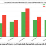 |
Figure 10: The mean efficiency metrics in both Dense Net systems with ML classifiers. |
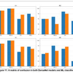 |
Figure 11: A matrix of confusion in both DenseNet models and ML classifiers. |
Comparing the State of the Art
As seen in table 14, results from the pre-trained DL models are displayed alongside earlier models employing MRI images. The employed method fared better than other earlier methods. In order to alter their effectiveness, this strategy combined pre-processing and ML classifier techniques with DenseNet-121 and DenseNet-201.
Table 14: Comparative Analysis with current Cutting-Edge Models.
| Reference | Dataset Used | No. of Images | Method | Accuracy |
| [6] | ADNI | 798 | VGG16, 2DCNN | 90.36% |
| [7] | ADNI | 3127 | 2DCNN with DL | 82.57% |
| [9] | ADNI | 1311 | CNN, k-NN, SVM | 75% |
| [10] | OASIS | 416 | PCA with FNN & DTCWT | 90.06% |
| [11] | ADNI | 1167 | CNN, SVM | 69.37% |
| [14] | ADNI | 1167 | SVM with DL | 75% |
| [15] | ADNI | 359 | CNN, SVM | 82.91% |
| [16] | OASIS | 416 | Cross Modal TL | 83.57% |
| [19] | ADNI | 1167 | CNN, SVM-REF | 81% |
| [22] | ADNI | 177 | ResNet50
DenseNet201 |
81.25%
84.38% |
| Suggested Method | Kaggle | 6400 | DenseNet201-SVM
DenseNet201-GNB DenseNet201-XGB |
91.02%
91.75% 91% |
Conclusion
This study demonstrated the significance of DL models in AD prediction. In a number of comparable metrics, DenseNet201 performs better than DenseNet121. Through Kaggle, the dataset was obtained. DenseNet201 for Gaussian NB produced the following results: 91.75% accuracy, 96.5% specificity, and 90.25% F1-score. For a variety of biomedical applications, medical imaging calls for different DL approaches. This model will be improved further in order to address problems with picture capture, improvement, integration of various data formats, and misalignment of weights when applying the model to particular AD concerns. The research’s significance may increase when more data are gathered. Additionally, a 3DCNN expansion, which focuses mostly on multimodal elements of brain MRI images, might be accomplished. GAN is used to supplement data may be put into practice as well. An alternative approach would be to employ reinforcement learning, which bases its judgments on the current environment. In order to attain more performance and openness, this strategy is currently being refined. The amount of AD imaging data and computer resources is increasing quickly, and this is driving constant change in the deep learning-based hybrid techniques for AD research. This would be a crucial benefit for both these applications and the novel techniques now used in healthcare facilities.
Acknowledgement
This paper was supported by KIIT Deemed to be University Library and Dr. Gopabandhu Sahu (Librarian), India, as well as the staff of SCB, Medical college, for their invaluable assistance and contributions to this study. Their dedication and support were integral to the successful completion of our study.
Funding Sources
The author(s) received no financial support for the research, authorship, and/or publication of this article
Conflict of Interest
The author(s) do not have any conflict of interest.
Data Availability
This statement does not apply to this article.
Ethics Statement
This research did not involve human participants, animal subjects, or any material that requires ethical approval.
Informed Consent Statement
This study did not involve human participants, and therefore, informed consent was not required.
Clinical Trial Registration
This research does not involve any clinical trials.
Permission to reproduce material from other sources
Not Applicable
Author’s Contribution
- Tulip Das: Conceptualization, Methodology, Writing – Original Draft
- Chinmaya Kumar Nayak: Visualization, Supervision
- Parthasarathi Pattnayak: Data Collection, Analysis, Writing – Review & Editing
Reference
- Adjei PO, Pattnayak P, Mohanty A, Das T, Patnaik S, Ansah P, Manneh M. Deep Learning for Alzheimer’s Diagnosis: ResNet152V2 Approach on MRI Dataset. In 2024 1st International Conference on Cognitive, Green and Ubiquitous Computing (IC-CGU). 2024; 1-6.
CrossRef - Ansah P, Pattnayak P, Mohanty A, Das T, Patnaik S, Adjei PO, Manneh M. Precision Medicine in Diabetes: A Machine Learning Model for Diabetic Foot Ulcer Prediction Using Keras TensorFlow. In 2024 1st International Conference on Cognitive, Green and Ubiquitous Computing (IC-CGU). 2024; 1-6.
CrossRef - Balaji P, Chaurasia MA, Bilfaqih SM, Muniasamy A, Alsid LE. Hybridized deep learning approach for detecting Alzheimer’s disease. Biomedicines. 2023;11(1);149.
CrossRef - Das T, Nayak CK, Pattnayak P. Improving the Detection of Alzheimer’s Disease with Advanced Artificial Diagnosis and Classification Methods. In 2024 International Conference on Inventive Computation Technologies (ICICT). 2024; 206-213.
CrossRef - Das T, Nayak CK, Pattnayak P. Alzheimer’s Disease Diagnosis Using Artificial Intelligence and MRI Images of the Brain. In 2024 3rd International Conference for Innovation in Technology (INOCON). 2024 ;1-6.
CrossRef - Xue C, Liu F, Chen H, et al. AI-based differential diagnosis of dementia etiologies on brain MRI. Nature Medicine. 2024; 30: 1410-1422.
CrossRef - Fleming A, Bourdenx M, Fujimaki M, et al. The different autophagy degradation pathways and neurodegeneration. Neuron. 2022;110(6):935-66.
CrossRef - Castellano G, D’Addabbo A, Mastronardi G, et al. Automated detection of Alzheimer’s disease: a multi-modal approach using MRI and amyloid PET (2D vs 3D). Scientific Reports. 2024; 14: 11809.
CrossRef - Lei B, Wang S, Chen C, et al. Alzheimer’s disease diagnosis from multi-modal data via feature inductive learning and dual multilevel graph neural network. Medical Image Analysis. 2024; 92: 103045.
CrossRef - Kang W, Lin L, Zhang B, Shen X, Wu S. Alzheimer’s Disease Neuroimaging Initiative. Multi-model and multi-slice ensemble learning architecture based on 2D convolutional neural networks for Alzheimer’s disease diagnosis. Computers in Biology and Medicine. 2021; (136):104678.
CrossRef - Krishna IM, Narsimham C, Chakravarthy AS. A hybrid machine learning framework for biomarkers based ADNI disease prediction. Ilkogr Online. 2021;(20):2532-2554.
- Lin Q, Che C, Hu H, Zhao X, Li S. A comprehensive study on early alzheimer’s disease detection through advanced machine learning techniques on mri data. Academic Journal of Science and Technology. 2023;8(1):281-285.
CrossRef - Leng Y, Cui W, Peng Y, et al. Alzheimer’s Disease Neuroimaging Initiative. Multimodal cross enhanced fusion network for diagnosis of Alzheimer’s disease and subjective memory complaints. Computers in Biology and Medicine. 2023;(157):106788.
CrossRef - Li Y, Fang Y, Wang J, Zhang H, Hu B. Biomarker extraction based on subspace learning for the prediction of mild cognitive impairment conversion. BioMed Research International. 2021;2021(1):5531940.
CrossRef - Zhang Y, Wu X, Liu Z, et al. Multi-modal graph neural network for early diagnosis of Alzheimer’s disease using phenotypic population graphs. Computers in Biology and Medicine. 2023; 157: 106825.
CrossRef - Pattnayak P, Mohanty A, Das T, Patnaik S. Applying Artificial Intelligence and Deep Learning to Identify Neglected Tropical Skin Disorders. In 2024 3rd International Conference for Innovation in Technology (INOCON). 2024;1-6.
CrossRef - Sadegh-Zadeh SA, Fakhri E, Bahrami M, et al. An approach toward artificial intelligence Alzheimer’s disease diagnosis using brain signals. diagnostics. 2023; 13(3):477.
CrossRef - Liu L, Zhang T, Xu K, et al. Cascaded Multi-Modal Mixing Transformers for Alzheimer’s disease classification. NeuroImage, 2023; 276: 120199.
CrossRef - Venugopalan J, Tong L, Hassanzadeh HR, Wang MD. Multimodal deep learning models for early detection of Alzheimer’s disease stage. Scientific reports. 2021;11(1):3254.
CrossRef - Xie C, Zhuang XX, Niu Z, et al. Amelioration of Alzheimer’s disease pathology by mitophagy inducers identified via machine learning and a cross-species workflow. Nature biomedical engineering. 2022;6(1):76-93.
CrossRef - Yao Z, Wang H, Yan W, et al. Artificial intelligence-based diagnosis of Alzheimer’s disease with brain MRI images. European Journal of Radiology. 2023; (165): 110934.
CrossRef - Yang Y, Arseni D, Zhang W, et al. Cryo-EM structures of amyloid-β 42 filaments from human brains. Science. 2022;375(6577):167-72.
CrossRef - Zhang J, He X, Liu Y, Cai Q, Chen H, Qing L. Multi-modal cross-attention network for Alzheimer’s disease diagnosis with multi-modality data. Computers in Biology and Medicine. 2023;162:107050.
CrossRef - Kim S-Y, Park J, Choi S, et al. Personalized explanations for early Alzheimer’s disease diagnosis using population-graph graph neural networks. IEEE Journal of Biomedical and Health Informatics. 2023; 27(7): 3129-3140.
- Gao X, Yin Y, Chen W, et al. Multimodal transformer network for incomplete image generation and Alzheimer’s disease diagnosis. Computers in Biology and Medicine. 2023; 158: 106896.

