Archana Saini^1*, Ayush Dogra²and Vinay Kukreja¹

¹Department of Computer Science and Engineering, Chitkara University Institute of Engineering and Technology, Chitkara University, Rajpura, Punjab, India

²Department of Electronics and Communication Engineering, Chitkara University Institute of Engineering and Technology, Chitkara University, Rajpura, Punjab, India.

Corresponding Author E-mail: saini.archana@chitkara.edu.in

 

DOI : https://dx.doi.org/10.13005/bpj/3216

Abstract

Medical imaging is essential for diagnosis and treatment planning, but different kinds of noise, such as Gaussian, Poisson, salt-and-pepper, and speckle noise, frequently degrades image quality. There are many radiological modalities, with each having its advantages and limitations, like MRI, CT, ultrasound, and X-ray, that provide useful information. Proper choice of radiation dosage to ensure high-quality images while reducing exposure risk is a significant issue in medical imaging. This study considers several denoising methods and assesses how well they work on datasets from magnetic resonance imaging (MRI) and high-resolution computed tomography (HRCT). Advanced deep-learning-based techniques like the denoising convolutional neural network (DnCNN) and block-matching and 3D filtering (BM3D) are contrasted with traditional techniques like bilateral filtering, guided filtering, and non-local means (NLM). The efficiency of denoising while maintaining anatomical features is evaluated by analyzing performance indicators such as peak signal-to-noise ratio (PSNR), structural similarity index (SSIM), and natural image quality evaluator (NIQE). The findings indicate that when compared with the other techniques, DnCNN and BM3D show better results while maintaining high visual clarity and structural fidelity. These results demonstrate the importance of selecting the appropriate denoising algorithm for the imaging modality and noise characteristics to enhance clinical decision-making and improve diagnostic accuracy.

Keywords

BM3D; Gaussian Noise; HRCT; Image Restoration; Medical Imaging; MRI

Download this article as: 

Copy the following to cite this article: Saini A, Dogra A, Kukreja V. From Spatial Domain to Learning Based Methods: A Survey on MRI and HRCT Image Denoising Methods. Biomed Pharmacol J 2025;18(3).

Copy the following to cite this URL: Saini A, Dogra A, Kukreja V. From Spatial Domain to Learning Based Methods: A Survey on MRI and HRCT Image Denoising Methods. Biomed Pharmacol J 2025;18(3).

Introduction

In medical imaging, image restoration is very important because the quality of visual information plays a great role in diagnosis and treatment planning. Among the major problems of image processing is the existence of noise that degrades image quality and hides useful features.¹ Several factors, including transmission problems, sensor technology limits, and environmental interferences, may cause noise in medical imaging.  Different types of noise adversely interfere with medical image quality and compromise the visual fidelity of crucial anatomy.² Therefore, an important objective in the area of medical image processing is to make medical images as good as possible using efficient denoising algorithms. An important reconstruction step is image denoising, which eliminates extraneous noise while preserving structural features.³ Different denoising strategies have been developed, ranging from conventional filtering-based techniques to sophisticated deep-learning-based systems. Each approach has its advantages based on the context of the application and the nature of the noise involved.⁴ Conventional techniques include linear as well as non-linear filtering: wavelet-based algorithms, median filtering, and Gaussian smoothing. Although these techniques reduce noise, they often blur or lose small features.⁵ Advanced methods of denoising arise as machine learning and artificial intelligence develop. Convolutional neural networks, generative adversarial networks, and autoencoders are some of the deep learning-based denoising algorithms that have done a great job in preserving the information while removing noise effectively.⁶ These are very successful in real-world applications as they are capable of adapting noise levels and realizing noisy patterns from big datasets. Despite these advantages, deep learning-based techniques may be limited in certain medical imaging applications due to their computational intensity and the training data that have to be correctly annotated.⁷

Medical images are subject to various noises, including speckle, salt-and-pepper, Poisson, and Gaussian noise. Gaussian noise manifests as random variations in pixel intensity and is often the result of electrical circuitry and thermal reasons.⁸ Poisson noise, also known as quantum noise, is related to photon counting statistics and is typical in low-light imaging environments. Salt-and-pepper noise, which is typically due to transmission faults or sensor failures, appears as scattered white and black pixels. Speckle noise is due to the coherent nature of wave reflection, is commonly observed in ultrasonography, and has a significant impact on image quality. Each form of noise requires the development of specialized filtering or learning-based algorithms for effective noise suppression .⁹ Effective denoising techniques are very important in medical imaging because they improve the quality and accuracy of pictures obtained from various imaging modalities. High-quality medical imaging results in better data analysis, which leads to more precise diagnoses and well-informed treatment choices. A more significant difficulty in denoising is maintaining delicate anatomical features while successfully eliminating noise. When denoising is insufficient, residual noises may remain that depreciate the ability to interpret correctly, but excessive smoothing leads to loss of fine features.¹⁰ Hence, the design of trustworthy denoising algorithms is a difficult research task that requires a kind of compromise between feature retention and noise reduction. The dependability of medical imaging will be further improved as technology develops through future advancements in denoising techniques, which will eventually improve clinical results and patient care.

Figure 1 demonstrates the basic steps that can be carried out during the denoising of an image. Firstly, an image is taken, then noise is added to the input image, and we get the noisy image. Then, various denoising algorithms can be applied, and as a result, a denoised image is produced.

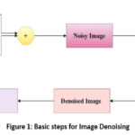Figure 1: Basic steps for Image Denoising Click here to view Figure

Literature Review

Suneetha et al. ¹¹ have proposed a modified fuzzy set filter to denoise the underwater photography fish dataset. A modified fuzzy set filter creates 24 fuzzy rules to locate the noisy pixels with an additional 4-pixel location. The extra eight fuzzy parameters make it easier to find the picture pixels irrespective of whether there is a need for averaging or not. Various levels of Gaussian noise (0.01, 0.03, and 0.1 levels) were employed to estimate the performance of the proposed model. Compared to traditional filtering techniques, the test results proved that the PSNR value improved by 2-3 dB. Tabatabaeefar et al. ¹² introduced a method that was tested on CT and MRI images through a combination of 2 algorithms: Genetic and Particle Swarm Optimization. Each image goes through various noises, such as Gaussian, speckle, and salt-and-pepper noise, in an attempt to create noise in two models. Around 5% of each noise type is mixed in the first model: speckle noise with a variance of 0.04, salt and pepper noise with a density of 0.05, and Gaussian noise with a variance of 0.01. Around 10% of each type of noise is mixed in the second model: Gaussian noise with a variance of 0.1, salt and pepper noise with a density of 0.1, and speckle noise with a variance of 0.1. For MRI and CT images, PSNR values varied between 59 and 63 and 63 and 65. Also, RMSE values varied between 12 and 20 for MRI and 36 and 47 for CT scans. A system of deep learning to denoise Gaussian noise from color and grayscale images is developed by Aghajarian et al. ¹³ There are three successive stages in the training procedure. The first stage is the training of a classifier to differentiate between noisy and clean images. In the second stage, a denoiser network removes noise from the image features that the classifier is trained to identify. Finally, the denoised features of the image are projected back to pixels in the image with a decoder. The performance is assessed using the BSDS68 (Berkeley segmentation dataset of 68 images) and 12 test images commonly used. The method achieves maximum PSNR at any level of noise for denoising BSDS68 grayscale images (large mean improvement of 0.99). The proposed method achieves the highest PSNR at all other noise levels (mean gain of 0.3) for color image denoising of BSDS68.  X-ray images were exposed to artificial noise simulation by Roy et al.,¹⁴ and a comparison experiment was performed to find out which filtering approach is better suited for which types of sounds. Ten images from the Kaggle chest X-ray imaging dataset were used. First, the images were exposed to Gaussian noise. Then, the images were filtered with Wiener, HMF, Anisotropic, Gaussian, and median filters. After applying Poisson Noise to the images, the same procedure was followed again. It was found that HMF Filtering performs very well for both noises. Also, anisotropic diffusion filtering performed well. However, no filter could be considered the best for both types of noise. Boby et al.¹⁵ test the performance of various denoising filtering methods. Based on the results, the best filter to denoise US, CT, or MRI images is the Gaussian filter. The median filtering method is better when reducing salt and pepper noise. The anisotropic diffusion filtering method is suggested to remove Poisson noise. Finally, the most appropriate filtering method to remove Gaussian noise is the non-local means. Deep and machine-learning methods have been employed by Sreelakshmi et al. ¹⁶ to detect brain-related diseases. A complex filter structure is needed for the rapid and accurate detection of brain diseases, as other filters, including Gaussian and median filters, are unable to remove noise when the noise is above 78%.  The adaptive median filter based on CNN-ML is proposed for effective disease detection and noise removal. The precision of MRI brain disease studies based on the CNN-AMF and GBML model is 0.9863. Singh et al.¹⁷ addressed the challenge of removing the harmful Gaussian additive white noise without distorting the important features. A CNN deep learning framework produces the proposed method. Gaussian noise is added at different noise variance levels (σ = 10, 15, 20, 25). The average computational time of the proposed method is 2.8760, the average PSNR value is 25.82, and its average SSIM value is 0.85. Yu et al. ¹⁸ calculated the SNR and PSNR values and analyzed the denoising effect of the Gaussian filter method on salt and pepper noise and Gaussian noise. After optimization, the SNR values for salt and pepper noise and Gaussian noise are 31.5896 and 57.69201, respectively. The PSNR of Gaussian noise is 31.5021, while that of salt and pepper noise is 19.7872. The denoising effect of the Gaussian filter on Gaussian noise is better than that of Salt and Pepper noise under the same conditions. Abuya et al.¹⁹ focused on the elimination of noise from CT scan images that were contaminated with additive Gaussian blur noise (AGBN) using an ensemble method that integrates a DnCNN with an anisotropic Gaussian filter (AGF) and wavelet transform. To eliminate AGBN, initially, denoising is done using the AGF and Haar wavelet transforms as preprocessing steps. To eliminate the residual noise, the DnCNN is then combined with AGF and wavelet for post-processing. The AGF is particularly used because it can adapt to directional information and edge orientation, avoiding blurring along edges in the case of non-uniform noise distribution. The proposed ensemble method has an average PSNR of 28.28 and an average computing time of 0.01666 s. The MSE value is very low, and the SSIM value is very close to 1.0. Sun et al. ²⁰ aimed to explore the denoising capability of low-dose myocardial perfusion (MP) SPECT based on a conditional generative adversarial network (cGAN) in the projection domain and reconstruction domain. The results indicate that cGAN denoising enhances image quality over LD and traditional filtering. It can also lower the dose level without affecting the image quality. The study concludes that cGAN-prj outperforms cGAN-recon for MP-SPECT. Priyadharsini et al. ²¹ have proposed a RAMF (Robust Adaptive Median Filter) approach for removing Salt and Pepper noise in breast cancer images. RAMF is a new filter approach where noise-free pixels are taken into account while calculating the median of the window. For good performance at high noise density, this approach uses a new method of initiating the picture reading from the center point. It applies an adaptive windowing strategy for filtering dense high densities of salt-and-pepper noise, with the size of the filtering window depending on the local density of noise. The filter performs well in low and medium density intervals (10%-90%), properly denoising higher density values. Sahu et al.²² proposed a model that applies the dual denoising network (DudeNet) model to chest X-rays (CXR) in medical image denoising (MID). The feature extraction is done with a sparse technique. The training is accelerated through batch normalization and residual learning to enhance denoising performance. There are five different levels of noise with σ = 15, 25, 40, 50, and 60 in CXR images. It is superior to the previously reported MID models. Mittal et al. ²³ proposed a deep residual learning model that does end-to-end mapping of noisy inputs to denoised outputs through the use of rectified linear unit activations and many residual learning blocks. Tested on 50 degraded photos, the proposed method outperformed the DCNN method, which had an average SSIM of 0.9811, with an SSIM of 0.9844 for mammography images. For X-ray image denoising, the model provides better PSNR and SSIM.CT and MRI are necessary diagnostic means for studying human anatomy and the properties of tissue. But they are still exposed to inherent and instrumental noises, including quantum mottle, Gaussian, and Rayleigh noises. Muthukrishnan et al. ²⁴ resolve this problem by applying the continuum topological derivative technique (CTD) method. The article experimented with different filters on HRCT and MR images and assessed their efficiency in removing the noise. The CTD technique was successful in eliminating quantum mottle noise in HRCT images as well as Gaussian and Rayleigh noise in MRI. The performance measures of the CTD technique were superior to all the other techniques. The results hold huge promise for exact diagnostic data in significant cases such as Thoracic Cavity Carina, Brain-Middle Cerebral Artery, neoplastic tumors, and Brain SPI Globe Lens 4th Ventricle. The efficiency of the U-Net architecture for lung CT image denoising with synthetically added Gaussian noise is tested by Park et al. ²⁵ Subsequently, utilizing measures such as MSE, PSNR, SSIM, and patch-based statistics differences’ skewness and kurtosis across a set of 100 CT DICOM files, set the noise standard deviations to 0.03, 0.05, and 0.07. The results exhibited significant enhancements in metrics evaluation post-denoising, showing the model’s ability to minimize noise and enhance diagnostic precision effectively. Annavarapu et al. ²⁶ proposed utilizing a deep modified CNN for image enhancement, image detail restoration via adaptive watershed segmentation, and hybrid lifting based on modified bi-histogram equalized contrast enhancement for image improvement. Subsequently, considering marker-based watershed segmentation, this process is further developed. The performance of this method is measured with the Jaccard Index, F1 score, and Dice Coefficient of the segmentation process, and PSNR, edge preservation index, contrast-to-noise ratio, Bhattacharya coefficient, and root mean square error of the image denoising approach. The proposed method comes up with a high PSNR measure of 43.76 dB at a value of standard deviation of 2 and a high value of Jaccard index measure of 0.95. A method of reducing Gaussian noise, speckle noise, salt and pepper noise, and ring artifacts in medical images, such as MRI, CT, and chest X-ray images, was presented by Annavarapu et al. ²⁷. To enhance image quality and deep learning-based Figure-Ground segmentation, this study explores the integration of adaptive CNNs with guided image filtering. The efficiency of the proposed method is extensively evaluated on chest X-ray and MRI/CT images under different conditions of noise, and the use of standard statistical parameters provides comparisons to alternative approaches. The results affirm that the proposed strategy outperforms, with each of these measures having the highest value. To remove noise from MRI, Juneja et al.²⁸ proposed an autoencoder-based network, Brain Tumor (BT)-Autonet. For the 128 × 128 image dataset, the proposed technique achieves a PSNR of 30.788, an MSE of 25.179, and an SSIM of 0.9 for the Gaussian dataset. With an execution time of 10.5 s for the Gaussian dataset, 11 s for the Rician dataset, and 11 s for the Rayleigh dataset, it achieves a PSNR of 27.952, MSE of 23.129, SSIM of 0.861 for the Rician dataset and PSNR of 25.329, MSE of 44.378, SSIM of 0.873 for the Rayleigh dataset. With an execution time of 25 s for the Gaussian Dataset, 27 s for the Rician Dataset, and 26 s for the Rayleigh Dataset, BT-Autonet has a PSNR of 30.452, MSE of 30.036, and SSIM of 0.816 for the Gaussian Dataset, 49.64, MSE of 41.684, SSIM of 0.809 for the Rician Dataset, and 12.818, MSE of 67.219, SSIM of 0.279 for the Rayleigh Dataset. An Efficient Transfer-Learning-Based Fractional Order (ETLFOD) image Denoising approach was released by Annadurai et al. ²⁹. Employing DenseNet121, this approach unites transfer learning with fractional order methods in a novel manner to address the requirements of medical image denoising. The accuracy, precision, and recall of the DenseNet121 model were 98.01%, 98%, and 98%, respectively. MRI brain datasets had 95% accuracy, 98% precision, 99% recall, and 96% F1-score, while COVID-19 lung data had 88% accuracy, 91% precision, 95% recall, and 88% F1-score. The X-ray pneumonia results of the lung CT dataset had 92% accuracy, 97% precision, 98% recall, and 93% F1-score.

Material and Methods

This section covers the details of the dataset used and the algorithms applied to it.

Dataset Description

There are two types of datasets used as input. The first dataset used HRCT images, whereas the second dataset contains MR images.^30-31

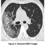Figure 2: Dataset1 (HRCT Image) Click here to view Figure

Figure 2 shows the dataset1, which is chest HRCT. In HRCT imaging, lung tissue is scanned in narrow slices of 1-2 mm, which enables minimal changes in the parenchyma and gives a relatively good portrayal of lung architecture. Its late phase is the most suitable for assessing lung conditions as it provides a higher resolution and contrast.

Figure 3: Dataset2 (MR Image) Click here to view Figure

The most likely sequence from the current MR imaging scan is the T1-weighted MRI sequence shown in Figure 3. In the T1-weighted picture, the gray matter of the brain is darker compared to the white matter, and the cerebrospinal fluid inside the ventricle is dark, too. This pattern is useful for detailing the architectural diversity of the human brain. It is mainly employed in high-resolution anatomical imaging to attain clear border demarcation between various brain areas.

Applied Different Noise Variances on the Dataset

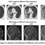Figure 4: Dataset1 and Dataset2 at different noise variances Click here to view Figure

Figure 4 shows dataset 1 (HRCT) and dataset 2 (MRI) at four different noise variances (0.01,0.05,0.09, and 0.5).

Applied Denoising Algorithms

Block-Matching and 3D Filtering (BM3D):

BM3D is a state-of-the-art method for image denoising using both collaborative filtering and the non-local mean. There exist two stages for the algorithm: Grouping and Collaborative filtering. Related image blocks are gathered from the entire data set according to a measure of similarity, and grouped into a three-dimensional array. Then, grouped patches undergo a transform-domain shrinkage, and then the denoised picture is reconstructed using an inverse transform. The primary thought is to largely suppress noise with no unacceptable loss of fine details by exploiting redundancy within as well as between comparable patches. BM3D is regarded as a current standard for picture denoising, and it is very good at cleaning away the Gaussian noise.³²

Expected Patch Log Likelihood (EPLL)

EPLL models the previous distribution of clean picture patches to use a probabilistic denoising technique. According to the approach, clean picture patches are taken from an earlier distribution, which is usually represented by Gaussian Mixture Models (GMMs). The anticipated log probability of patches under the prior distribution is maximized to produce the denoised picture. To prevent artifacts, patches are processed in overlapping windows, and the final image is reassembled using weighted averaging. EPLL works well with a variety of noise types because it strikes a compromise between data quality and previous knowledge.³³

Fields of Experts (FoE)

FoE uses learned filter banks as the prior model and is based on the Markov Random Field (MRF) technique. The method combines responses from a set of learned convolutional filters to form a prior over the entire image. Filters are learned to capture local textures and structures. The denoising procedure combines a data fidelity term and the learnt prior term to minimize an energy function. FoE is very efficient in noise elimination while keeping up the textures and edges.³⁴

Weighted Nuclear Norm Minimization (WNNM)

WNNM is a denoising algorithm using low-rank approximation. Its main steps are given as follows: Patches related are combined into the matrix. There is a row in the matrix corresponding to every patch. The matrix SVD (singular value decomposition) operation is performed. SVD values are compressed using weighted nuclear norm reduction on their weights so that noise gets reduced. This method works well with images that have periodic patterns and can tolerate some amount of organized noise.³⁵

Bilateral Filtering

This is a very simple yet powerful edge-preserving denoising algorithm. It works by averaging the pixels based on intensity similarity and geographic proximity. Weights are assigned to the pixels in the neighborhood, and these weights decline with increasing spatial distance and difference in intensity. The bilateral filter performs well up to moderate levels of noise and is computationally inexpensive.³⁶

Guided Filtering

Guided filtering enhances bilateral filtering by using a guiding image that controls the filtering process. A linear model is obtained to describe the filtering operation based on the guided image. This model is used to enhance the features and edges of the noisy image. This method is often used on picture fusion and edge-preserving smoothing tasks.³⁷

Non-Local Means (NLM)

This non-local denoising method depends on the image patches’ self-similarity properties. It computes the weighted average for every pixel of a picture by employing weights from values of similarities the patches carry amongst themselves. A patch closer in similarity to a target patch would then take a larger weight. It has the computation cost, though in the end, it still works properly and also allows for the effective removal of noises while holding to details very precisely.³⁸

Denoising Convolutional Neural Network (DnCNN)

DnCNN is an image denoising algorithm that utilizes deep learning. Its architectural features include: Batch normalization and ReLU activation in convolutional layers. The output of the noisy image is the difference between the noisy image and the noise obtained using a residual learning framework for noise forecasting. DnCNN is flexible and works well with a variety of noise levels and types.³⁹

Bayesian NLM

Bayesian NLM extends NLM by using Bayesian inference to estimate the weights. It uses past information to model the probability that a pixel is part of a clean patch. It refines the denoising procedure using the posterior probability. This method increases accuracy and resilience in high-noise situations.⁴⁰

Adaptive Clustering and Principal Component Analysis for Texture (ACPT)

ACPT aims to denoise textured regions through adaptive cluster formation of similar patches. PCA is then applied to the clustered patches to retain textures while reducing the noise. It is quite effective on the photographs with dense texture. ⁴¹

Adaptive Clustering and Variance Analysis (ACVA)

ACVA performs denoising by using variance analysis to group patches to manage different noise levels. It grouped patches by using adaptive filtering to reduce the noise effectively. Images with non-uniform distributions of noise might benefit from the ACVA.⁴²

Adaptive Sparse Transform and Non-Local Self-Similarity (AST_NLS)

This technique combines ideas of non-local self-similarity and sparse coding. First, learn the adaptive sparse transform to represent patches. Then group the patches for collaborative processing. This technique works better in preserving structures and textures.

Non-Locally Centralized Sparse Representation (NCSR)

NCSR integrates non-local patch grouping and sparse coding. Its process involves extracting patches and non-locally classifying similar ones. It reduces noise through centralized restrictions and sparse representation. NCSR is capable of handling complex patterns and textures.⁴³

Total Variation L1 Norm (TVL1)

TVL1 is a variational denoising method that suppresses the total variation of the image. It develops an energy function with a total variance regularization term and an L1 norm fidelity term. It solves the optimization problem by using numerical methods. TVL1 is robust against high noise values and performs satisfactorily in edge-preserving denoising. ⁴⁴

Results

In this section, the performance of various denoising algorithms has been evaluated at four different noise variances based on various performance metrics, such as PSNR, entropy, SSIM, MSE, NIQE, BRISQUE, and PIQE.

Table 1: Performance evaluation of different algorithms at different noise variances for dataset 1

Algorithms	N.V	Entropy	PSNR	MSE	SSIM	NIQE	BRISQUE	PIQE
TVL1	0.01	0.99	10.33	27205.70	0.000015	7.82	43.46	42.80
	0.05	0.99	10.33	27207.62	0.000011	7.43	42.19	63.67
	0.09	0.99	10.33	27208.14	0.000009	7.43	36.14	66.02
	0.5	0.99	10.32	27213.15	0.000005	7.54	37.78	74.65
NLM	0.01	6.97	24.31	241.84	0.45	8.24	32.55	47.41
	0.05	6.87	21.50	471.41	0.31	10.22	42.83	62.59
	0.09	6.93	19.85	691.07	0.25	19.55	43.44	66.08
	0.5	6.87	14.41	2429.23	0.10	60.52	43.46	75.69
BayesianNLM	0.01	6.941	23.536	319.570	0.502	6.174	34.752	46.621
	0.05	7.469	17.549	1186.205	0.325	15.979	44.516	67.775
	0.09	7.521	14.591	2281.806	0.229	24.584	45.391	71.809
	0.5	7.093	8.220	9826.570	0.067	93.747	43.458	82.852
BM3D	0.01	7.14	25.45	185.44	0.54	5.16	13.90	39.99
	0.05	7.13	22.67	351.77	0.32	4.13	11.87	35.70
	0.09	7.21	21.80	430.02	0.28	4.84	10.37	36.10
	0.5	7.56	19.02	813.15	0.17	6.10	10.78	38.15
EPLL	0.01	7.14	25.25	195.46	0.52	4.61	1.94	30.76
	0.05	6.71	21.76	443.02	0.29	8.30	32.30	45.44
	0.09	6.75	20.15	646.57	0.23	10.06	42.74	48.23
	0.5	6.62	14.09	2619.92	0.06	66.36	43.46	65.30
Guided	0.01	7.17	20.51	579.96	0.22	7.24	48.31	70.60
	0.05	7.22	19.67	711.44	0.20	8.14	47.54	63.77
	0.09	7.23	18.90	861.92	0.19	8.54	46.93	58.53
	0.5	7.05	14.75	2273.92	0.11	8.98	45.23	43.25
DnCNN	0.01	7.19	25.37	189.80	0.56	4.05	24.16	35.86
	0.05	7.07	22.06	416.07	0.38	6.20	23.93	39.63
	0.09	7.10	20.30	627.83	0.32	7.69	27.64	38.81
	0.5	7.31	14.26	2530.92	0.16	60.90	43.78	64.93
WNNM	0.01	7.33	22.72	187.96	0.63	4.96	30.60	51.65
	0.05	6.99	26.76	483.53	0.38	8.42	30.91	48.58
	0.09	6.49	27.34	557.23	0.28	4.74	13.56	44.13
	0.5	7.19	33.69	2415.21	0.15	43.60	44.37	73.72
Bilateral	0.01	7.34	23.49	291.99	0.51	8.42	39.29	27.71
	0.05	7.51	20.96	532.50	0.39	9.65	41.28	22.64
	0.09	7.58	19.31	780.48	0.33	10.07	42.83	21.62
	0.5	7.52	14.05	2659.48	0.17	14.30	43.38	25.04
ACPT	0.01	7.34	25.29	225.51	0.62	8.44	36.39	54.76
	0.05	7.13	21.00	563.86	0.40	13.16	41.12	59.82
	0.09	6.50	20.03	703.08	0.29	4.61	9.58	31.05
	0.5	7.00	13.61	2968.73	0.13	95.19	43.48	77.05
AST_NLS	0.01	7.34	25.44	216.47	0.62	7.18	34.65	51.00
	0.05	7.15	21.24	536.39	0.39	11.12	40.19	55.22
	0.09	6.47	20.68	616.70	0.30	7.94	33.99	41.21
	0.5	7.07	14.38	2508.25	0.14	63.35	43.47	73.91
ACVA	0.01	7.44	25.08	203.23	0.64	8.03	36.42	58.37
	0.05	7.19	21.06	518.61	0.40	10.09	40.83	61.89
	0.09	6.66	20.15	646.31	0.27	3.68	16.99	37.12
	0.5	7.14	13.77	2817.42	0.14	66.92	43.49	79.15
NCSR	0.01	7.47	24.64	223.46	0.61	7.03	34.45	52.34
	0.05	7.47	20.82	537.92	0.34	7.03	34.45	52.34
	0.09	7.47	20.50	579.54	0.26	7.03	34.45	52.34
	0.5	7.47	14.15	2502.68	0.12	7.03	34.45	52.34
FoE	0.01	7.70	23.19	312.81	0.60	12.66	40.60	64.15
	0.05	7.88	15.55	1824.00	0.29	27.19	50.08	76.32
	0.09	7.78	13.11	3196.34	0.20	31.12	56.09	78.27
	0.5	7.00	8.07	10245.80	0.07	80.40	43.46	85.27

Table 1 depicts the performance evaluation of different algorithms at different noise variances for dataset 1.BM3D maintains steady feature retention of the image because of slight changes in the entropy with increased noise variance (7.14 at N.V. 0.01 to 7.56 at N.V. 0.5). PSNR indicates reduced noise suppression effectiveness as noise levels increase, dropping from 25.45 at N.V. 0.01 to 19.02 at N.V. 0.5. With noise, MSE increases significantly (from 185.44 to 813.15), indicating a greater deviation from the original image. SSIM exhibits a loss of structural similarity at increasing noise levels, which falls from 0.54 to 0.17. Good perceptual quality is achieved by perceptual metrics (NIQE, BRISQUE, PIQE) as scores are generally low (for instance, NIQE ranges from 5.16 to 6.10). At higher noise levels, EPLL entropy drops slightly (7.14 at N.V 0.01 to 6.62 at N.V 0.5), indicating a slight information loss. Its poor performance at high noise levels is also evident from the sharp drop in PSNR from 25.25 to 14.09. The high increase in MSE indicates more distortion that varies from 5.46 to 2619.92, and SSIM indicates poor structural retention and drops sharply from 0.52 to 0.06. Perceptual measures like BRISQUE and PIQE both decrease, signifying low visual quality, while NIQE sharply increases (4.61 to 66.36). The FoE technique with the highest entropy of 7.70 at N.V. 0.01 depicts excellent texture preservation but drops down at high noise levels. At high noise levels, PSNR is not suitable, MSE increases exponentially (312.81 to 10245.80), and SSIM depicts poor structural preservation and remains low (0.60 to 0.07). High NIQE and BRISQUE scores indicate deteriorated perceptual quality. WNNM’s entropy ranges from 7.19 at N.V. 0.5 to 7.33 at N.V. 0.01, which is stable and moderate. At first, PSNR is good (22.72 at N.V. 0.01) but degrades at increasing noise levels (33.69 at N.V. 0.5). MSE shows a growing deviation with noise, ranging from 187.96 to 2415.21. SSIM declined moderately (0.63 to 0.15). NIQE ranged from 4.96 to 43.60, indicating mixed performance.  DnCNN shows consistent entropy (0.19 at N.V. 0.01 to 7.31 at N.V. 0.5). It also shows excellent performance in PSNR, demonstrating noise-adaptability (25.37 to 14.26), but MSE moderately rises from 189.80 to 2530.92. It also maintains an SSIM value between 0.56 and 0.16, indicating strong structural preservation. Perceptual metrics like NIQE and BRISQUE continue to be competitive when compared against alternative approaches. At every noise level, bilateral shows higher entropy (7.34 at N.V. 0.01 to 7.52 at N.V. 0.5), and MSE also increases constantly from 291.99 to 2659.48. PSNR: Does only a fair job (23.49 to 14.05). It maintains structural similarity by reducing SSIM values from 0.51 to 0.17. It achieves a high PIQE score that shows excellent visual quality. At low noise, the guided filtering entropy is moderate, but at high noise, it significantly reduces. PSNR values are not good (20.51 to 14.75). MSE increases significantly from 579.96 to 2273.92. All the noise levels have a low SSIM (0.22 to 0.11). High NIQE and PIQE scores indicate poorer visual quality. Bayesian NLM entropy is stable but slightly drops at high noise levels (6.941 to 7.093). It shows low performance in terms of PSNR (23.536 to 8.220). There is exponential growth in MSE (319.570 to 9826.570). SSIM shows structural degradation as it declines (0.502 to 0.067). Perceptual metrics like BRISQUE and NIQE score high at high noise levels. Good detail retention is demonstrated by the high entropy values maintained by ACVA and AST_NLS. In terms of PSNR, TVL1 suffers at all noise levels, whereas ACPT does well at low noise levels but degrades at higher ones. TVL1’s MSE is noticeably high, indicating that it is not appropriate for denoising. SSIM denotes that TVL1 performs quite poorly, although ACPT and ACVA maintain structure rather well. When compared to other methods, ACVA and AST_NLS retain acceptable perceptual quality. The low perceptual metric scores and high PSNR of BM3D and DnCNN make them the most resilient for all noise levels. With low PSNR and high NIQE scores, FoE and TVL1 perform badly, especially at higher noise levels. Although WNNM and EPLL provide balanced performance, they are less effective in very noisy environments.

Table 2: Performance evaluation of different algorithms at different noise variances for dataset 2    

Algorithms	N.V	Entropy	PSNR	MSE	SSIM	NIQE	BRISQUE	PIQE
TVL1	0.01	0.33	14.11	4696.88	0.0256	5.22	40.84	38.63
	0.05	0.33	14.11	4697.55	0.0223	5.42	38.60	56.68
	0.09	0.31	14.11	4698.14	0.0236	6.09	44.76	66.57
	0.5	0.29	14.10	4700.32	0.0207	7.00	36.97	72.85
NLM	0.01	6.33	30.64	64.61	0.33	9.77	39.14	53.71
	0.05	6.49	24.94	284.49	0.19	10.99	43.42	62.22
	0.09	6.51	23.20	495.67	0.15	12.19	43.46	65.91
	0.5	6.40	18.23	2438.70	0.07	47.04	43.46	76.40
BayesianNLM	0.01	6.850	24.16	437.960	0.373	10.409	38.920	53.423
	0.05	7.154	16.72	1748.841	0.178	23.614	50.946	73.623
	0.09	7.192	13.63	3286.207	0.121	37.775	43.693	76.296
	0.5	6.452	8.397	11258.88	0.039	102.06	43.458	84.904
BM3D	0.01	6.50	35.72	17.44	0.48	5.2	36.74	57.01
	0.05	6.53	31.10	50.45	0.36	5.59	27.53	49.32
	0.09	6.53	29.38	75.04	0.31	5.74	26.98	46.77
	0.5	6.57	24.18	248.5	0.18	5.97	27.52	44.78
EPLL	0.01	6.34	32.06	52.88	0.44	7.65	23.50	50.68
	0.05	6.43	26.08	272.65	0.30	10.30	35.02	53.42
	0.09	6.44	23.98	512.32	0.24	10.83	43.45	58.80
	0.5	6.19	18.22	2642.52	0.10	33.71	43.46	70.93
Guided	0.01	6.58	29.98	78.03	0.44	7.84	49.36	56.39
	0.05	6.71	25.60	292.96	0.31	8.28	50.44	45.95
	0.09	6.75	23.82	525.91	0.26	8.69	49.54	42.60
	0.5	6.62	18.56	2566.24	0.13	9.50	44.46	34.01
DnCNN	0.01	6.46	31.27	60.75	0.39	4.15	10.18	36.57
	0.05	6.63	25.60	285.06	0.25	4.79	19.60	37.40
	0.09	6.69	23.48	538.33	0.20	5.99	20.89	39.31
	0.5	6.88	17.09	2891.19	0.06	38.74	43.49	61.55
WNNM	0.01	6.15	16.98	58.30	0.36	6.21	24.74	55.31
	0.05	6.29	23.25	296.70	0.22	7.00	32.91	54.90
	0.09	6.06	23.06	386.19	0.25	6.96	32.16	60.30
	0.5	6.44	30.16	2461.04	0.06	24.54	43.51	74.00
Bilateral	0.01	6.81	30.11	76.17	0.35	6.79	40.93	25.64
	0.05	7.00	23.91	376.38	0.21	8.74	42.60	20.67
	0.09	7.06	21.83	682.93	0.16	9.10	43.19	18.74
	0.5	7.17	16.60	3071.97	0.07	12.80	43.43	19.80
ACPT	0.01	5.99	28.37	104.30	0.48	7.68	31.50	38.11
	0.05	6.20	22.58	475.95	0.29	10.49	30.99	44.30
	0.09	6.56	21.67	696.74	0.27	10.80	45.01	54.40
	0.5	6.60	15.98	3358.62	0.09	71.58	48.37	73.91
AST_NLS	0.01	6.09	28.72	93.74	0.487378	7.97	25.04	50.87
	0.05	6.38	23.22	386.25	0.313032	11.60	31.75	50.85
	0.09	6.04	22.81	526.45	0.277818	11.10	35.09	60.58
	0.5	6.48	17.16	2633.21	0.108643	57.02	43.74	71.97
ACVA	0.01	6.06	30.18	75.97	0.35	4.70	24.95	47.74
	0.05	6.20	23.84	387.81	0.20	5.99	29.45	48.57
	0.09	6.23	23.99	525.11	0.26	4.81	37.12	54.56
	0.5	6.62	16.78	3082.25	0.05	17.64	46.42	79.08
NCSR	0.01	6.27	28.76	86.43	0.50	5.47	42.43	48.94
	0.05	6.27	22.96	329.27	0.34	5.47	42.43	48.94
	0.09	6.27	21.46	464.94	0.27	5.47	42.43	48.94
	0.5	6.27	14.10	2529.77	0.10	5.47	42.43	48.94
FoE	0.01	6.99	25.28	206.06	0.21	12.78	43.01	64.14
	0.05	7.22	16.45	1583.62	0.07	19.88	48.43	74.74
	0.09	7.24	13.85	2936.89	0.04	24.99	45.17	78.09
	0.5	6.82	8.65	10548.27	0.01	69.14	43.46	85.00

A comparison of many denoising methods based on different performance measures for dataset 2 is shown in Table 2. The evaluation of varying denoising algorithms shows that BM3D gives the highest PSNR, 35.72 at N.V. 0.01 and 24.18 at N.V. 0.5, of all the methods, which suggests better quality in noise removal. Low MSE values confirm noise reduction with precision, and SSIM values ranging between 0.48 and 0.18 depict excellent structural preservation. Also, lower NIQE, BRISQUE, and PIQE scores reflect high perceptual quality. EPLL, by contrast, is worse and yields lower PSNR and SSIM values while significantly raising MSE (from 52.88 at N.V. 0.01 to 2642.52 at N.V. 0.5), which indicates very poor noise suppression. FoE has high entropy but fails at high noise levels as it shows a sharp PSNR drop from 25.28 to 8.65 and an extremely high rise in MSE 10548.27 at N.V. 0.5, thus making it a completely non-performing denoise tool. WNNM is significantly good at low noise levels; however, the values of PSNR and SSIM reduce for it at higher noise levels, and its perceptual scores are better than FoE but poorer than BM3D. The bilateral filter achieves middle-level PSNR and SSIM values; it does better than FoE but slightly worse than BM3D. The high MSE increase with the increase in noise variance brings down its overall efficiency, though very low PIQE values do suggest good perceptual quality for real-world images. Guided filtering remains competitive in PSNR, but high BRISQUE and NIQE scores indicate that it doesn’t work well in perceptual quality. NLM is good at low noise but degrades quickly with increasing noise, so it is not as handy in applications with high noise levels. DnCNN is ranked second only to BM3D: its PSNR and MSE values confirm the effectiveness of noise suppression, and its perceptual scores remain favourable, so DnCNN is a particularly strong alternative. The Bayesian NLM failed with high levels of noise: PSNR low, MSE large, and the value of SSIM dropped steeply, affirming its vulnerability in preserving structural details. The performances of PSNR and SSIM of ACPT, ACVA, and AST_NLS were moderate, while the MSE became larger with the increase of higher noise. ACVA has superior perceptual quality to the rest of the considered techniques. NCSR keeps SSIM and PSNR at relatively constant but modest values, while perceptual evaluations are a little worse than BM3D, but its MSE is controlled. TVL1 is the worst algorithm as it suffers from extreme distortion of images because of its highest MSE and lowest PSNR values. Furthermore, because its SSIM is approaching zero, structural details are lost, and poor visual quality is confirmed by its perceptual scores. It has been observed that BM3D is the best denoising algorithm, with strong perceptual quality, low MSE, and high PSNR, making it a very effective tool for noise suppression. DnCNN is an effective deep learning-based alternative, with superior performance in both quality and perceptual measures. TVL1 is the weakest of the methods and performs poorly on all metrics. FoE and Bayesian NLM are ineffective in high-noise conditions, while ACPT, ACVA, and AST_NLS are viable alternatives in certain noise environments. This study confirms that BM3D and DnCNN are the most suitable denoising algorithms for clinical imaging, excelling in numerical accuracy and perceptual quality, respectively.

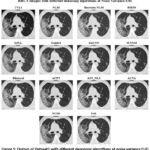Figure 5: Output of Dataset1 with different denoising algorithms at noise variance 0.01 Click here to view Figure

Figure 5 presents HRCT images denoised by various algorithms at a Noise Variance (N.V.) of 0.01. The performance of each algorithm in noise reduction and structural preservation is quite different, as shown in the figure. Among these methods, BM3D shows the best performance, maintaining sharp edges and preserving fine details while effectively suppressing noise. Similarly, DnCNN, a deep-learning approach, also presents a high-quality balance between noise reduction and detail preservation. Its performance is close to that of BM3D. The image remains sharp with clear edges and minimal blurring.  WNNM shows effective noise suppression but causes the loss of some texture details compared with BM3D and DnCNN. EPLL shows good denoising power but looks over-smoothed, resulting in the loss of finer anatomical structures, which may affect clinical interpretations. Guided Filtering shows visible noise reduction but also introduces some level of blurring, which is detrimental to the clarity. Though the lung structures are still separable, they are not as sharp as in BM3D or DnCNN. Similarly, Bilateral Filtering provides a moderate level of denoising but still exhibits some graininess, and edges appear less sharp compared to BM3D or WNNM. Other methods like ACPT, AST_NLS, and ACVA show reasonable noise removal capabilities. Their ability to preserve structural details varies, though. Among these, ACVA seems to provide the best perceptual quality. NLM and Bayesian NLM are known to work fairly well for low noise variance but result in low-level blurring while reducing noise. On the other hand, FoE produces a noisier result, which is not sharp and cannot suppress noise well, and the image looks less clear than those processed with BM3D or DnCNN. NCSR provides moderate performance but with some blurring and loss of texture details. Finally, TVL1 is the worst-performing algorithm in this set, causing severe loss of structural information. The result seems over-smoothed with misaligned details, and so it cannot be used in medical applications.

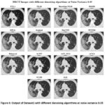Figure 6: Output of Dataset1 with different denoising algorithms at noise variance 0.05 Click here to view Figure

Figure 6 shows the denoised HRCT images using a variety of algorithms at a Noise Variance (N.V.) of 0.05. Among the methods, BM3D remains one of the best-performing techniques, effectively suppressing noise while maintaining fine anatomical structures with clear contrast. DnCNN also demonstrates strong performance, preserving sharp edges and lung structures while reducing noise, making it a reliable deep-learning-based denoising approach. WNNM continues to have the denoising capability without significant noise reduction but the loss in the fine details. Guided Filtering and EPLL significantly remove the noise, but the amount of over-smoothing diminishes the visibility of the small lung structures. Bilateral Filtering gives medium denoising performance but continues to exhibit a lot of noise artifacts with the blurring of fine details. ACPT, AST_NLS, and ACVA balance noise removal with structural preservation, with ACVA producing relatively clearer results. However, Bayesian NLM and NLM (Non-Local Means) suffer at the cost of noise variance with increased graininess, but a lesser sharpness level. Noisiness is more prevalent with FoE and NCSR than with other techniques since they cannot successfully remove the noise while retaining structural integrity. The worst one was TVL1 (Total Variation L1 Norm), highly over-smoothing and anatomically distorted. As the noise variance increases to 0.05, BM3D and DnCNN continue to demonstrate the best balance between noise suppression and structural preservation, making them the most effective choices for medical imaging. WNNM and ACVA offer moderate results but still introduce some loss of fine details. In contrast, TVL1, FoE, and Bayesian NLM struggle to produce clinically viable outputs due to excessive blurring or retained noise artifacts. At higher values of noise, deep learning types such as DnCNN and advanced filtering types like BM3D are more preferred in medical imaging, where anatomical structures have to be preserved for precise diagnosis.

Figure 7 indicates a large amount of noise. It shows HRCT scans denoised using different techniques at a Noise Variance (N.V.) of 0.09, making the denoising procedure even more difficult. The capacity of each method to reduce noise while maintaining precise anatomical features differs significantly as the noise variance rises. One of the best results is still being achieved by BM3D, effectively reducing the noise while maintaining lung architecture with sharp edges and high contrast. In the same way, DnCNN works satisfactorily in terms of providing some adequate balance between the reduction of noise and the structure-preserving but at the cost of highly over-smoothing. WNNM succeeds in denoising but makes some finer details harder to spot, making certain anatomical structures difficult to discern. At this noise level, Bayesian NLM has large residual noise and therefore appears grainy, whereas Non-Local Means and Bayesian NLM have a problem. The images get blurred by guided filtering and EPLL leads to a significant decrease in the small features of the lung function visualization since these methods also reduce noise to a certain extent. The sharpness and denoising would have to be traded off because, though quite famous for edge retention, bilateral filtering suffers in the case of increased noise. ACPT, AST_NLS, and ACVA even though still reasonable at denoising, preserve more features while reducing noise; ACVA does a little better at this. TVL1 is one of the poorer methods that over-smoothes the image with a significant loss in structural information and several distortions. FoE and NCSR both perform poorly; FoE is particularly weak in noise removal, resulting in an overwhelmingly grainy output with plenty of noise artifacts. Generally, BM3D and DnCNN are still the best algorithms for HRCT denoising at higher noise variance, striking a perfect balance between preserving structure and noise reduction. WNNM and ACVA have mediocre results and hence are not ideal for medical imaging applications. Among the worst are TVL1, Bayesian NLM, and FoE.

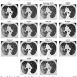Figure 7: Output of Dataset1 with different denoising algorithms at noise variance 0.09 Click here to view Figure

Figure 8 demonstrates the performance of various denoising techniques at a very high noise variance of 0.5 and, it has been observed that, except for the BM3D method, all algorithms yield fuzzy images. However, the output of the BM3D algorithm is not fully satisfactory. Therefore, none of the methods have been proven to be effective with a noise variance of 0.5.

Figure 9 shows a comparative evaluation of various denoising techniques on MRI images at a low Noise Variance (N.V.) of 0.01. BM3D is one of the best options for the medical picture denoising technique, performing very well, preserving delicate anatomical features with low noise artifacts and good contrast. DnCNN comes next and accurately finds a proper balance between removing noise and retention of features and provides sharp edges with soft features. WNNM denoises well, but it has a small quantity of smoothing involved, which results in a fine loss of detailed structural features. Bayesian NLM and NLM both provide fairly modest denoising, while Bayesian NLM retains more of the noise, creating a gritty impression of the image. EPLL and guided filtering are effective methods for noise reduction, but may slightly over-smoothed the data, hiding the small features. Bilateral filtering is not a good noise reducer compared to BM3D or DnCNN, although it provides edge-aware noise reduction. ACPT, AST_NLS, and ACVA show reasonable performance, while ACVA still maintains a good trade-off between anatomical clarity and noise reduction. TVL1 led to excessive smoothing that lost much structural information. FoE and NCSR can hardly eliminate the noise. FoE becomes somewhat grainy because of leftover noise. In all the compared algorithms, it can be concluded that ACPT highly reduced image quality most likely because of excessive processing. However, the highest-quality denoising performance came from BM3D and DnCNN which not only had successfully removed noises from MRI images but also have kept essential anatomical features preserved while Bayesian NLM, TVL1, and FoE perform the poorest.

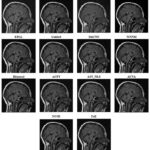Figure 8: Output of Dataset1 with different denoising algorithms at noise variance 0.5 Click here to view Figure

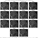Figure 9: Output of Dataset2 with different denoising algorithms at noise variance 0.01 Click here to view Figure

Figure 10 shows the denoised images using several methods at a noise of 0.05. BM3D is still among the topmost-ranking denoising techniques; the methods reduce the noise effectively while preserving the fine features of anatomy with high-quality texture and contrast. DnCNN is also a reliable choice for MRI image denoising since it also achieves a good trade-off between noise removal and feature preservation. Both WNNM and NLM perform well, but NLM leaves a bit more residual noise than WNNM. On the other hand, Bayesian NLM suffers from higher noise variance and results in a very grainy image with significant residual noise distortions. The performance of guided filtering, EPLL, and bilateral filtering is mediocre; they successfully reduce noise but also acquire a little smoothing effect that may cause fine details to be lost. Although ACPT may reduce the image quality because of the loss of structures, ACVA and AST_NLS are robust in producing visually clear images and keeping the details of the original structure. On the other hand, TVL1 is efficient in denoising images, but with an over-smoothing effect such that the remaining important contrast and texture are vanished. This makes FoE and NCSR be the weakest among the list of algorithms here. NCSR results in extreme blurring, which compromises the structural integrity of the image and reduces its diagnostic value. Guided filtering, EPLL, and bilateral filtering perform poorly; they can remove noise but have a small amount of smoothing effect that may lead to loss of fine details.

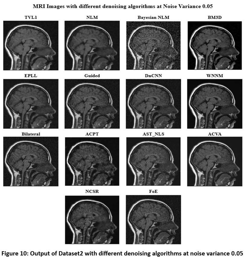Figure 10: Output of Dataset2 with different denoising algorithms at noise variance 0.05 Click here to view Figure

Figure 11: Output of Dataset2 with different denoising algorithms at noise variance 0.09 Click here to view Figure

Figure 11 depicts several denoising algorithms at a high noise variance of 0.09. BM3D is one of the most successful algorithms among them because it saves many anatomical features in the image with accuracy as well as retains high picture clarity. Other such effective models include DnCNN and WNNM, both of which return very sharp pictures with almost zero blur and intense contrast preservation. Bayesian NLM performs miserably and results in a highly noised image with significant graininess. Though NLM produces a good decrease in noise at this noise variance, the residue graininess would make it less suitable for application in clinics at this variance. Guided filtering, EPLL, and bilateral filtering over smoothed the image and, hide the small features. While ACPT produces a blurred output, which reduces the interpretability of pictures, ACVA and AST_NLS find a reasonable balance between denoising and structure preservation. TVL1 suppresses noise well but is over-smoothed, losing important medical information. In this high-noise environment, NCSR and FoE perform worse. While FoE fails to effectively reduce noise, leading to a grainy and less useful output.

Figure 12: Output of Dataset2 with different denoising algorithms at noise variance 0.5 Click here to view Figure

In Figure 12, MRI scans with a noise variance of 0.5 are shown, which has been denoised by several different methods. The relative performance of different denoising algorithms varies greatly as the noise variance is increased. Although no denoising algorithms perform well as the noise variance increases, every algorithm gives blurred images as the output, and these blurred images are not helpful in diagnosing the disease.

Discussion

Various algorithms perform adequately in diverse noise levels, some methods doing well in low-noise environments while others struggle with larger noise changes. At high noise variances, traditional filtering techniques such as bilateral filtering, guided filtering, and NLM are prone to blurring or not completely removing noise, even though they have decent performance in denoising. While Bayesian NLM is good at low levels of noise, it is poor at high levels of noise and yields unstable results that obscure diagnosis. Similarly, methods like FoE and TVL1 do not work well, particularly at high noise levels, and result in either over-smoothing or under-suppression of noise. While there are some algorithms, like WNNM and EPLL, that perform denoising effectively, they do tend to over-smooth images, potentially complicating the visualization of fine anatomical details. ACPT, AST_NLS, and ACVA; ACVA performs slightly better at maintaining features while denoising. FoE and NCSR are the worst-performing algorithms. Since FoE has a lot of noise retained, the image becomes very grainy-looking and is less suitable for medical interpretation. Nevertheless, NCSR induces severe blurring, which compromises the structure of the image and makes it less diagnostic. The main challenge in denoising strategies is that remove noise without compromising on information that has clinical importance. The best denoising approach is always BM3D, which produces wonderful images with minimal loss of structural details. It is particularly apt for applications in medical imaging, where accuracy matters the most due to its ability to find a middle ground between removing noise and maintaining features. Another deep learning approach known as DnCNN works well too, particularly in addressing different types and levels of noise. It is a competitive choice to BM3D due to its ability to adapt to various levels of noise, especially considering automatic denoising in clinical applications. The results emphasize that there is no single technique that performs optimally in all cases and that the imaging modality, anticipated noise variability, and diagnostic requirement must all be considered when choosing an algorithm. The most promising avenue for enhancing denoising performance in medical imaging is the integration of deep learning-based, adaptive, and noise-aware methods.

Conclusion

Denoising is an essential step in medical image processing, which aims to enhance diagnostic accuracy without affecting structural integrity. The study systematically assessed various denoising algorithms on HRCT and MRI datasets at different noise variances. Results show that BM3D consistently offers the best noise suppression with minimal structural distortion, which is why it becomes the optimal choice for medical image enhancement. DnCNN also delivers high performance, offering strong adaptability across noise levels due to its deep-learning framework. Conventional filtering methods, such as bilateral and guided filtering, perform reasonably well at lower noise levels but struggle with significant noise variance, leading to image blurring and loss of critical details. Bayesian NLM, FoE, and TVL1 exhibit poor performance, particularly in high-noise environments, making them less suitable for clinical applications. Future research should focus on developing hybrid denoising techniques that leverage machine learning and traditional methods to achieve the optimal balance between noise reduction and anatomical preservation. In conclusion, the study indicates that BM3D and DnCNN are the most effective denoising algorithms for real clinical imaging use, particularly for HRCT and MRI. Healthcare professionals can enhance patient care, reduce interpretation errors, and enhance diagnostic outcomes by implementing these findings into imaging procedures.

Acknowledgement
The authors are grateful to Chitkara University for the doctoral fellowship and its support.

Funding Source

The authors received no financial support for the research, authorship, and/or publication of this article.

Conflict of Interest

The authors do not have any conflict of interest.

Data Availability Statement

The dataset used in this study is open-source and freely available.

Ethics Statement

This research did not involve human participants, animal subjects, or any material that requires ethical approval.

Informed Consent Statement

This study did not involve human participants, and therefore, informed consent was not required.

Permission to reproduce material from other sources

This study did not use reproduced material from other sources.

Clinical Trial Registration

This research does not involve any clinical trials.

Author Contributions

• Archana Saini: Conceptualization, Methodology, Writing – Original Draft.
• Ayush Dogra: Data Collection, Analysis, Writing – Review & Editing.
• Vinay Kukreja: Visualization, Supervision.

References

1. Sagheer SVM, George SN. A review on medical image denoising algorithms. Biomedical Signal Processing Control. 2020; 61:102036.
   CrossRef
2. Cui H, Hu L, Chi L. Advances in computer-aided medical image processing. Applied Sciences. 2023;13(12):7079.
   CrossRef
3. Liu F, Song Q, Jin G. The classification and denoising of image noise based on deep neural networks. Applied Intelligence. 2020;50(7):2194-2207.
   CrossRef
4. Goyal B, Dogra A, Agrawal S, Sohi BS, Sharma A. Image denoising review: From classical to state-of-the-art approaches. Information fusion. 2020;55:220-244.
   CrossRef
5. Ilesanmi AE, Ilesanmi TO. Methods for image denoising using convolutional neural network: a review. Complex & Intelligent Systems. 2021;7(5):2179-2198.
   CrossRef
6. Liu F, Song Q, Jin G. The classification and denoising of image noise based on deep neural networks. Applied Intelligence. 2020;50(7):2194-2207.
   CrossRef
7. Jifara W, Jiang F, Rho S, Cheng M, Liu S. Medical image denoising using convolutional neural network: a residual learning approach. The Journal of Supercomputing. 2019; 75:704-718.
   CrossRef
8. Salami AM, Salih DM, Fadhil AF. Thermal image features and noise effects analysis. 7th International Engineering Conference “Research & Innovation amid Global Pandemic”(IEC). 2021; 2021:43-47.
   CrossRef
9. Jain A, Ingle M. Performance analysis of noise removal techniques for facial images—a comparative study.
10. Charmouti B, Junoh AK, Abdurrazzaq A, Mashor MY. A new denoising method for removing salt & pepper noise from image. Multimedia Tools and Applications. 2022;81(3):3981-3993.
    CrossRef
11. Suneetha A, Srinivasa Reddy E. Robust Gaussian noise detection and removal in color images using modified fuzzy set filter. Journal of intelligent systems. 2020;30(1):240-257.
    CrossRef
12. Tabatabaeefar M, Mostaar A. Biomedical image denoising based on hybrid optimization algorithm and sequential filters. Journal of biomedical physics & engineering. 2020;10(1):83.
    CrossRef
13. Aghajarian M, McInroy JE, Muknahallipatna S. Deep learning algorithm for Gaussian noise removal from images. Journal of Electronic Imaging. 2020;29(4):043005.
    CrossRef
14. Roy A, Maity P. A comparative analysis of various filters to denoise medical X-ray images. 4th International Conference on Electronics, Materials Engineering & Nano-Technology (IEMENTech).  2020;1-5.
    CrossRef
15. Boby SM, Sharmin S. Medical image denoising techniques against hazardous noises: an IQA metrics based comparative analysis. International Journal of Image, Graphics and Signal Processing. 2021;14(2):25.
    CrossRef
16. Sreelakshmi D, Inthiyaz S. Fast and denoise feature extraction based ADMF–CNN with GBML framework for MRI brain image. International Journal of Speech Technology. 2021;24(2):529-544.
    CrossRef
17. Singh P, Diwakar M, Gupta R, et al. A method noise-based convolutional neural network technique for CT image denoising. Electronics. 2022;11(21):3535.
    CrossRef
18. Yu J. Based on Gaussian filter to improve the effect of the images in Gaussian noise and pepper noise. Journal of Physics: Conference Series. Vol 2580. IOP Publishing; 2023:012062.
    CrossRef
19. Abuya TK, Rimiru RM, Okeyo GO. An image denoising technique using wavelet-anisotropic Gaussian filter-based denoising convolutional neural network for CT images. Applied sciences. 2023;13(21):12069.
    CrossRef
20. Sun J, Jiang H, Du Y, et al. Deep learning-based denoising in projection-domain and reconstruction-domain for low-dose myocardial perfusion SPECT. Journal of Nuclear Cardiology. 2023;30(3):970-985.
    CrossRef
21. Priyadharsini MS, Sathiaseelan JGR. The new robust adaptive median filter for denoising cancer images using image processing techniques. Indian J Sci Technol. 2023;16:35.
    CrossRef
22. Sahu A, Rana KPS, Kumar V. An application of deep dual convolutional neural network for enhanced medical image denoising. Medical & Biological Engineering & Computing. 2023;61(5):991-1004.
    CrossRef
23. Mittal A, Kaur N, Gupta A, Singh G. Deep residual learning-based denoiser for medical X-ray images. Evolving Systems. 2024;15(6):2339-2353.
    CrossRef
24. Muthukrishnan V, Jaipurkar S, Damodaran N. Continuum topological derivative—a novel application tool for denoising CT and MRI medical images. BMC Medical Imaging. 2024;24(1):182.
    CrossRef
25. Park CY, Jo B. Quantitative evaluation of a deep learning-based U-Net model for denoising lung CT images. Journal of Magnetics. 2024;29(4):550-557.
    CrossRef
26. Annavarapu A, Borra S. An adaptive watershed segmentation based medical image denoising using deep convolutional neural networks. Biomedical Signal Processing and Control. 2024;93:106119.
    CrossRef
27. Annavarapu A, Borra S. Figure-ground segmentation based medical image denoising using deep convolutional neural networks. International Journal of Computers and Applications. 2024;46(12):
    CrossRef
28. Juneja M, Rathee A, Verma R, et al. Denoising of magnetic resonance images of brain tumor using BT-Autonet. Biomedical Signal Processing and Control. 2024; 87:105477.
    CrossRef
29. Annadurai A, Sureshkumar V, Jaganathan D, Dhanasekaran S. Enhancing medical image quality using fractional order denoising integrated with transfer learning. Biomedical Signal Processing and Control. 2024;8(9):511.
    CrossRef
30. Image Fusion, Image Denoising, Image Enhancement. GitHub. https://github.com/Imagingscience/Image-Fusion-Image-Denoising-Image-Enhancement-. Accessed March 6, 2025.
31. Harvard Medical School. Whole Brain Atlas. https://www.med.harvard.edu/aanlib/home.html. Accessed March 6, 2025.
32. Mahmood SZ, Afzal H, Mufti MR, et al. A novel method of image denoising: new variant of block matching and 3D. Journal of Medical Imaging and Health Informatics. 2020;10(10):2490-2500.
    CrossRef
33. Ali R, Yunfeng P, Amin RU. A novel Bayesian patch-based approach for image denoising. IEEE Access. 2020; 8:38985-38994.
    CrossRef
34. R S VK. FOE NET: segmentation of fetal in ultrasound images using V-NET. International journal of electrical and computer engineering systems. 2023;14(10):1141-1149.
    CrossRef
35. Mahaboob Basha S, Neto AVL, Menezes JWM, et al. Evaluation of weighted nuclear norm minimization algorithm for ultrasound image denoising. Wireless Communications and Mobile Computing. 2022;3167717.
    CrossRef
36. Vinodhbabu P, Swapna P. A hybrid method for denoising of medical images using DWT and bilateral filter. International Journal of Research in Engineering, IT and Social Sciences. 2019;09(5):27-36.
37. Altaie RH. Restoration for blurred noisy images based on guided filtering and inverse filter. International Journal of Electrical and Computer Engineering (IJECE). 2021;11(2):1265-1275.
    CrossRef
38. Liu C, Zhang L. A novel denoising algorithm based on wavelet and non-local moment mean filtering. Electronics. 2023;12(6):1461.
    CrossRef
39. Shaliniswetha S, Mahaboob ST. Residual learning based image denoising and compression using DnCNN. ICTACT Journal on Image & Video Processing. 2022;13(2).
    CrossRef
40. Arora P, Singh P, Girdhar A, Vijayvergiya R. Performance analysis of various denoising filters on intravascular ultrasound coronary artery images. International Journal of Imaging Systems and Technology. 2023;33(3):965-984.
    CrossRef
41. Li P, Wang H, Li X, Zhang C. An image denoising algorithm based on adaptive clustering and singular value decomposition. IET Image Processing. 2021;15(3):598-614.
    CrossRef
42. Kamesh Iyer S, Moon BF, Josselyn N, et al. Quantitative susceptibility mapping using plug-and-play alternating direction method of multipliers. Scientific Reports. 2022;12(1):21679.
    CrossRef
43. Fan L, Zhang F, Fan H, Zhang C. Brief review of image denoising techniques. Visual computing for industry, biomedicine, and art. 2019;2(1):7.
    CrossRef
44. Fang L, Xianghai W. Adaptive total-variation and nonconvex low-rank model for image denoising. International Journal of Image and Graphics. 2023; 25:2550016.
    CrossRef