M. Merlin and B. Priestly Shan

¹Research Scholar, Sathyabama University,Chennai ²Principal, Royal College of Engineering and Technology, Thrissur, Kerela

DOI : https://dx.doi.org/10.13005/bpj/865

Abstract

Automated techniques for eye diseases identification are very important in the ophthalmology field. Conventional techniques for the identification of retinal diseases are based on manual observation of the retinal components (optic disk, macula,  vessels, etc.). This paper presents a new supervised method for blood vessel detection in digital retinal images. This method uses a Fuzzy logic based Support Vector Machine  scheme for pixel organization and computes a 5-D vector composed of gray-level and intensity histogram-based features for pixel representation. The method was evaluated on the  publicly  available  DRIVE  and  STARE  databases,  widely used for this intention since they contain retinal images where the vascular structure has been precisely marked by experts. Its effectiveness and robustness with different image conditions, together with its simplicity and fast implementation, make this blood vessel segmentation proposal suitable for retinal image computer analyses such as automated screening for early diabetic retinopathy detection.

Keywords

Diabetic retinopathy; GLCM; retinal imaging; telemedicine; vessels segmentation

Download this article as: 

Copy the following to cite this article: Merlin M, Shan B. P. Robust and Efficient Segmentation of Blood Vessel in Retinal Images using Gray-Level Textures Features and Fuzzy SVM. Biomed Pharmacol J 2015;8(1)

Copy the following to cite this URL: Merlin M, Shan B. P. Robust and Efficient Segmentation of Blood Vessel in Retinal Images using Gray-Level Textures Features and Fuzzy SVM. Biomed Pharmacol J 2015;8(1). Available from: http://biomedpharmajournal.org/?p=2012>

Introduction

Recent advances in computer technology have enabled the progress of numerous types of Computer-Aided Medical Diagnosis – CAMD – over the years. Currently, medical image analysis is a research area that attracts a lot of concern from both scientists and physicians. Computerized medical imaging and analysis methods using multiple modalities have facilitated early diagnosis, treatment evaluation, and therapeutic intervention in the clinical  management of critical diseases[1]. DIABETIC retinopathy (DR) is the leading ophthalmic pathological cause of blindness among people of working age in developed countries. It is motivated by diabetes-mellitus complications and, although diabetes warmth does not necessarily involve vision impairment, about 2% of the patients affected by this disorder are blind and 10% undergo vision degradation after 15 years of diabetes, as a consequence of DR complications. The estimated prevalence of diabetes for all age groups worldwide was 2.8% in 2000 and 4.4% in 2030, meaning that the total number of diabetes patients is forecasted to rise from 171 million in 2000 to 366 million in 2030 [2].

Several automated techniques have been reported to quantify the  changes in morphology of retinal vessels (width, tortuosity) indicative of retinal or cardiovascular diseases. Some of the techniques measure the vessel morphology as an  average value representing the entire vessel network, e.g., average tortuosity [3]. However  recently, vessel morphology  measurement  specific to arteries or  veins was found to  be  associated with disease. For example, ‘plus’ disease in retinopathy of prematurity (ROP) may result in increase in arterial tortuosity relative to that of veins indicating the need for preventative treatment [4]. Arterial narrowing, venous dilatation, and resulting decrease in artery-to- venous width ratio (AVR) may predict the future occurrence of a stroke event or a myocardial infarct [5]. Unfortunately, the detection of minute changes in vessel width or tortuosity specific to arteries or  veins may be difficult in a  visual evaluation by an ophthalmologist or by a semi-automated method, which is laborious in clinical practice. Therefore, an automated identifica- tion and separation of individual vessel trees and the subsequent classification into arteries and veins is required for vessel specific morphology analysis [6].

Blood vessels appeared as networks of either deep red or orange-red filaments that originated within the optic disc and were of progressively diminishing width. Several approaches for extracting retinal image vessels have been developed which can be divided as; one consists of supervised classifier-based algorithms and the other utilizes tracking-based approaches. Supervised classifier-based algorithm usually comprise of two steps. First, a low-level algorithm produces segmentation of spatially connected regions. These candidate regions are then classified as vascular or non-vascular. The application of mathematical morphology and wavelet transform was investigated for identification of retinal blood vessels [7]. In a follow-up study, a two-dimensional Gabor wavelet was utilized to initially segment the retinal images.

A Bayesian classifier was then applied to classify extracted feature vectors as vascular or non-vascular. Tracking-based approaches utilize a profile model to incrementally step along and segment a vessel. Vessel tracking proceeded iteratively from the papilla, halting when the response to a one-dimensional matched filter fell below a given threshold. The tracking method was driven by a fuzzy model of a one-dimensional vessel profile [8]. One drawback to these approaches is their dependence upon methods for locating the starting points, which must always be either at the optic nerve or at subsequently detected branch points. Blood vessels were detected by means of mathematical morphology [9]. Matched filters were applied in conjunction with other techniques such as genetic algorithms and piecewise thresholding [10]. The rest of the article are described as follows, the proposed blood vessel segmentation method is presented in section 2, the experimental results are presented in section 3 and the conclusion in section 4.

Proposed Method for Vessel classification

This paper proposes a new supervised approach for blood vessel detection based on a NN for pixel classification. The essential feature vector is computed from preprocessed retinal images in the neighborhood of the pixel under consideration. The following process stages may be identified: 1) original fundus image pre-processing for gray-level homogenization and blood vessel enhancement, 2) feature extraction for pixel numerical representation, 3) application of a classifier to label the pixel as vessel or nonvessel, and 4) post-processing for filling pixel gaps in detected blood vessels and removing falsely-detected secluded vessel pixels. Input images are monochrome and obtained by extracting the green band from original RGB retinal images. The green channel provides the best vessel-background contrast of the RGB-representation, while the red channel is the brightest color channel and has low contrast, and the blue one offers poor dynamic range. Thus, blood containing elements in the retinal layer (such as vessels) are best represented and reach higher contrast in the green channel [11].

All parameters described below were set by experiments carried out on DRIVE images with the aim of contributing the best segmentation performance on this database (performance was evaluated in terms of average accuracy—a detailed description is provided in Sections V-A and V-B). Therefore, they refer tom retinas of approximately 540 pixels in diameter. The application of the methodology to retinas of different size (i.e., the diameter in pixels of STARE database retinas is approximately 650 pixels) demands either resizing input images to complete this condition or adapting proportionately the whole set of used parameters to this new retina size.

Preprocessing

Color fundus images often show imperative lighting variations, poor contrast and noise. In order to reduce these imperfections and generate images more suitable for extracting the pixel features demanded in the classification step, a preprocessing comprising the following steps is applied: 1) vessel central light reflex removal, 2) background homogenization, and 3) vessel enhancement. Next, a description of the procedure, illustrated through its application to a STARE database fundus image (Fig. 1), is detailed.

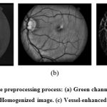Figure 1: Illustration of the preprocessing process: (a) Green channel of the original image. (b) (b) Homogenized image. (c) Vessel-enhanced image. Click here to view full figure

 

Color fundus images often show important lighting variations, poor contrast and noise. In order to decrease these imperfections and generate images more suitable for extracting the pixel features demanded in the classification step, a pre- processing comprising the following steps is applied: 1) vessel central light reflex removal, 2) background homogenization, and 3) vessel enhancement.

Vessel Central Light Reflex Removal

Since retinal blood vessels have lesser reflectance when compared to other retinal surfaces, they appear darker than the background. Although the typical vessel cross-sectional gray-level profile can be approximated by a Gaussian shaped curve (inner vessel pixels are darker than the outermost ones), some blood vessels include a light streak (known as a light reflex) which runs down the central length of the blood vessel. To remove this brighter strip, the green plane of the image is filtered by applying a morphological opening using a three-pixel diameter disc, defined in a square grid by using eight connexity, as structuring element. Disc diameter was fixed to the probable minimum value to reduce the risk of merging close vessels.

Background Homogenization

Fundus images often contain background intensity variation due to non uniform illumination. Consequently, background pixels may have different intensity for the same image and, even though their gray-levels are usually higher than those of vessel pixels (in relation to green channel images), the intensity values of some background pixels is equivalent to that of brighter vessel pixels. Since the feature vector used to represent a pixel in the classification stage is formed by gray-scale values, this effect may worsen the performance of the vessel segmentation methodology. With the purpose of removing these background lightening variations, a shade-corrected image is accomplished from a background estimate. This image is the result of a filtering operation with a large arithmetic mean kernel,

Vessel Enhancement

The final pre-processing step consists on generating a new vessel-enhanced image, Vessel enhancement is performed by estimating the complementary image of the homogenized image and subsequently applying the morphological Top-Hat transformation. The pre-processing results of two images with different illumination condition are shown in figure 2.

 

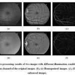Figure:2 pre processing results of two images with different illumination conditions. (a), (d) Green channel of the original images. (b), (e) Homogenized images. (c), (f) Vessel-enhanced images. Click here to view full figure

 

Feature Extraction

The aim of the feature extraction stage is pixel characterization by means of a feature vector, a pixel representation in terms of some quantifiable measurements which may be easily used in the classification stage to decide whether pixels belong to a real blood vessel or not. In this paper, the following sets of features were selected. These features are: Laplacian of Gaussian (LoG), gray level co-occurrence matrix (GLCM) and directional Gabor texture features (DGTF). The features extracted are discussed below:

Laplacian of Gaussian (LoG)

LoG filters at Gaussian widths of 0.25, 0.50, 1, and 2 are considered. These values are convoluted with the input image. Sixteen features are retrieved by calculating mean, standard deviation, skewness, autocorrelation, busyness, coarseness and kurtosis for the LoG filter output in the SROI region.

Mean

The mean (m) is defined as the sum of the intensity values of pixels divided by the number of pixels in the SROI of an image.

Standard Deviation

It shows how much variation or exists from the expected value i.e., the mean. The data points tend to be very close to the mean results low standard deviation and the data points are spread out over a large range of values results high standard deviation.

Skewness

It is a measure of the asymmetry of the data around the sample mean. If the value is negative, the data are spread out more to the left of meaner than to the right. If the value is positive, the data are spread out more to the right. The sickness of the normal distribution (or any perfectly symmetric distribution) is zero. The skewness of a distribution is defined as

Y=E(x-µ)³/σ³                                       

Where µ is the mean of x, σ is the standard deviation of x, and E(t) represents the expected value of the quantity t.

Autocorrelation

It is used to evaluate the quantity of promptness as well as the excellence of the texture present in the image, denoted as f(δi, δj). For a n x m image is defined as follows:

 

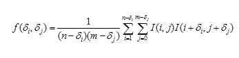
Here 1 ≤ δi  ≤ n and 1 ≤ δj  ≤ m. δi  and δj  represent a shift on rows and columns, respectively.

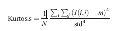
Kurtosis

The forth central moment gives kurtosis. It gives the measure of closeness of an intensity distribution to the normal Gaussian shape.

 

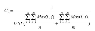
Coarseness

The Coarseness is calculated based on the Shape. This value is not equal to zero then the segmented area has been affected by the tumor, otherwise the tumor does not affect the segmented area. It is the average number of maxima in the autocorrelated images and original images.  The coarseness (Cs) is calculated as follows

Busyness

It is calculated based on connectivity, how much the pixels are connected is calculated that is above 5 then the segmented area has a tumor. The business’ value is below 5 the segmented area does not have a tumor. The Busyness value is depending on Coarseness .If the value of Coarseness is high ,the  It is related to coarseness in the reverse order, that is when the business is low.

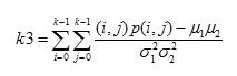
Gray Level Co-Occurrence Matrix

Gray-level-based features: features based on the differences between the gray-level in the candidate pixel and a statistical value representative of its surroundings. It contains the second-order statistical information of neighboring pixels of an image. It is estimated of a joint probability density function (PDF) of gray level pairs in an image [12].

It can be expressed in the following equation

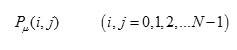
Where  i , j indicate the gray level of two pixels ,N is the gray image dimensions ,μ is the position relation of two pixels .Different values of μ decides the distance and direction of two pixels .Normally Distance (D) is 1,2 and Direction(θ) is 00,450,900,1350 are used for calculation [13 ].

Texture features can be extracted from gray level images using GLCM Matrix .In our proposed method ,five texture features energy, contrast, correlation , entropy  and homogeneity are experiments. These features are extracted from the segmented MR images and analyzed using various directions and distances.

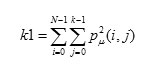
Energy expresses the repetition of pixel pairs of an image

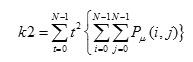
Local variations present in the image is measured  by Contrast.   If the contrast  value is high means the image has large variations.

Correlation is a measure linear dependency of gray level values in co-occurrence matrices. It is a two dimensional frequency histogram in which individual pixel pairs are assigned to each other on the basis of a specific ,predefined displacement vector

 

Where μ_¹,μ₂,σ₁,σ₂   are  mean  and  standard  deviation values accumulated in the x and y directions respectively.

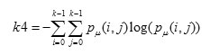
Entropy is a measure of non-uniformity in the image based on the probability of      Co- occurrence values, it also indicates the complexity of the image

 

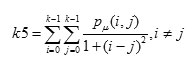
Homogeneity is inversely proportional to contrast at constant energy whereas it is inversely proportional to energy

 

Directional Gabor Texture Features (DGTF)

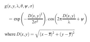
Directional Gabor’s are used as they measure the heterogeneity in the SROI. Gabor filter is a Gaussian kernel function modulated by a sinusoidal plane wave. There-fore, it gives directional texture features at a specified Gaussian scale. Gabor kernel is defined as:

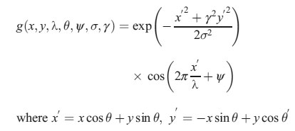
In this equation, λ represents the wavelength of the sinusoidal factor, θ represents the orientation of the normal to the parallel stripes of a Gabor function, ψ is the phase offset, σ is the width of the Gaussian, and γ is the spatial aspect ratio, and specifies the ellipticity of the support of the Gabor function [14]. The intensity and texture features summary is given in Table 1.

Rotation Invariant Circular Gabor Features (RICGF)

Gabor filter is a Gaussian kernel function modulated by a radially sinusoidal surface wave; therefore, it gives rotational invariant texture features which are given by:

 

Where, λ represents the wavelength of the sinusoidal factor, θ represents the orientation of the normal to the parallel stripes of a Gabor function, ψ is the phase offset, σ is the width of the Gaussian, and γ is the spatial aspect ratio, and specifies the ellipticity of the support of the Gabor function.

 Table: 1  Summary Of Intensity And Texture Features

Feature Category	Features	Number of Features
LoG	Four statistical parameters for the LoG filter output in the SROI region are retrieved at σ = 0.25, 0.50, 1, and 2 thereby contributing 16 features in the feature pool. These parameters are: (1) mean intensity, (2) standard deviation, (3) Skewness, (4) Kurtosis	16 features
GLCM	Following GLCM features at 0°, 45°, 90°, and 135° are calculated: (1) contrast, (2) homogeneity, (3) correlation, (4)Energy	4*4 =16 features
DGTF	RICGFs are calculated  at λ for 2√2, 4, 4√2, 8, 8√2) and θ for 0°, 22.5°, 45°, 67.5°, and 90° are varied. Four statistical parameters are calculated for each filter output in the marked SROI  and are taken as 100 features in the feature bank. These parameters are: (1) mean intensity, (2) standard deviation, (3) Skewness, (4) Kurtosis	25* 4=100 features
RICGFs	RICGFs are calculated at λ =2√2, 4, 4√2, 8, 8√2) and two values of ψ, i.e., 0° and 90° four statistical parameters for each filter output in the marked SROI and are taken as 40 features in the feature bank. These features are: (1) mean intensity, (2) standard deviation, (3) Skewness, (4) Kurtosis	10* 4=40 features

 

Classification using FSVM

The SVM has been widely used in pattern recognition applications due to its computational efficiency and good generalization performance. It is widely used in object detection and recognition, content-based image retrieval, text recognition, biometrics, speech recognition, etc. It creates a hyperplane that separates the data into two classes with the maximum margin. Originally it was a linear classifier based on the optimal hyperplane algorithm .A support vector machine searches an optimal separating hyper-plane between members and non-members of a given class in a high. In SVMs , the training process is very sensitive to those training data points which are away from their own class.  In our proposed method Fuzzy logic based SVM (FSVM) is applied for classification .It is an effective supervised classifier and accurate learning technique, which was first proposed by Lin and Wang [17]. In FSVM is to assign each data point a membership value according to its relative importance in the class. Since each data point  has an assigned membership value, the training set and is given by

For positive class , the set of membership values are denoted as , and are denoted as   for negative class , they are assigned independently. The main process of fuzzy SVM is to maximize the margin of separation and minimize the classification error.

The optimal hyperplane problem of FSVM can be defined as the following problem [15,16].

 

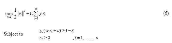
Where f_i (_{^{0≤ f}i} ≤1) is the fuzzy membership function f _ie _i, is a error of different weights and C is a constant

The inputs to FSVM algorithm are the feature subset selected via Enhanced TCM. It follows the structural risk minimization principle from the statistical learning theory. Its kernel is to control the practical risk and classification capacity in order to broaden the margin between the classes and reduce the true costs . A Fuzzy support vector machine searches an optimal separating hyper-plane between members and non-members of a given class in a high dimension feature space .

The Lagrange multiplier function of FSVM is

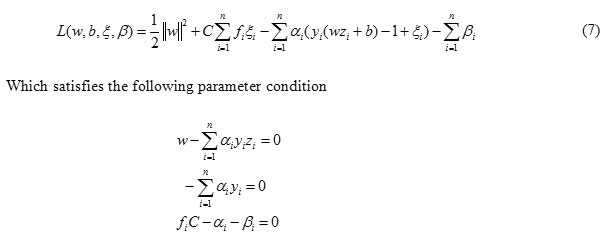
Then the optimization problem can be transferred to

Where the parameter   can be solved by the sequential minimal optimization (SMO) quadratic programming approach [18].In Nonlinear data , the input space X can be mapped into higher dimensional feature space . It’s become linearly separable. The mapping function   should be in accordance with Mercer’s theorem [19].

It can be chosen from the following functions

Polynomial learning machine kernel function

FSVM Training and Testing Process

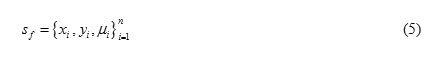
To train and testing  the Fuzzy SVM classifier, we need some data features to identify the vessel region or not. The data features will then train the classifier and the classifier will find the vessel region in the retinal image. The data features which we have chosen for training the FSVM classifier are concatenated of the  172 features (Detailed in section 2.2).

Experimental Results

Performance Measures

In order to quantify the algorithmic performance of the proposed  method on a fundus image, the resulting segmentation is compared to its corresponding gold-standard image. This image is obtained by manual creation of a vessel mask in which all vessel pixels are set to one and all nonvessel pixels are set to zero. Thus, automated vessel segmentation performance can be assessed. In this paper, our algorithm was evaluated in terms of Sensitivity , Specificity ,Positive Predictive Value(PPV), Negative Predictive Value(NPV) and Accuracy [20]. It is defined as follows

Sensitivity = TP/(TP+FN)

Specificity = TN/(TN+FP)

PPV = TP/(TP+FP)

NPV = TN/ (TN+FN)

Accuracy = (TN+TP)/(TN+TP+FN+FP)

Sensitivity and specificity metrics are the ratio of well-classified vessel and nonvessel pixels, respectively.  Positive predictive value is the ratio of pixels classified as vessel pixel that are correctly classified. Negative predictive value is the ratio of pixels classified as background pixel that are correctly classified. Finally, accuracy is a global measure providing the ratio of total well-classified pixels. The Contingency Vessel Classification is given in Table II.

Table: 2 Contingency Vessel Classification

Proposed Method Evaluation

This method was evaluated on DRIVE and STARE database images with available gold-standard images. Since the images’ dark background outside the FOV is easily detected. Sensitivity , specificity, positive predictive value , negative predictive value and accuracy values were computed for each image considering FOV pixels only. Since FOV masks are not provided for STARE images, they were generated with an approximate diameter of 650    550. The results are listed in Tables III and IV.

Table: 3 Performance Results  On Drive Database  Images

Image	Sensitivity	Specificity	PPV	NPV	Accuracy
1	59.97	98.44	82.45	95.27	94.25
2	87.81	96.75	76.03	98.54	95.81
3	77.96	97.70	82.46	96.97	95.30
4	77.65	97.87	83.74	96.87	95.37
5	69.10	98.50	85.98	95.99	95.04
6	68.02	98.25	86.39	94.97	94.02
7	70.39	98.82	89.26	95.99	95.34
8	58.40	99.61	91.72	96.98	96.75
9	67.76	98.72	76.94	97.99	96.89
10	69.44	98.19	82.27	96.59	95.26

A vessel was considered thin if its width is lower than 50% of the width of the widest optic disc vessel. Otherwise the vessel is considered non-thin. On the other hand, a FP    is considered to be far from a vessel border if the distance from its nearest vessel border pixel in the gold-standard is over two pixels. Otherwise, the FP is considered to be near. Table IV summarizes the results of this study. This table shows the average ratio of FN           and      FP provided by the segmentation algorithm for the 10 test images in the DRIVE and STARE databases. The average percent of        FN  and FP     corresponding to the different spacial locations considered are also shown. For both databases, the percent of        FN produced in non-thin vessel pixels was higher than that in thin vessel pixels.

Table: 4 Performance Results  On Stare Database  Images

Image	Sensitivity	Specificity	PPV	NPV	Accuracy
1	81.09	97.24	76.01	97.95	98.67
2	87.81	96.75	76.03	98.54	95.81
3	77.96	97.70	82.46	96.97	95.30
4	77.65	97.87	83.74	96.87	95.37
5	69.10	98.50	85.98	95.99	95.04
6	68.02	98.25	86.39	94.97	94.02
7	70.39	98.82	89.24	95.99	95.34
8	58.40	99.61	91.72	96.98	96.75
9	67.76	98.72	76.94	97.99	96.89
10	62.25	97.63	72.45	96.27	94.41

 

The experimental results of sensitivity, specificity ,PPV,NPV and accuracy of  DRIVE data base is shown in Figure 3 and STARE data base is shown in Figure 4.

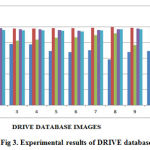Figure 3: Experimental results of DRIVE database Click here to view full figure

 

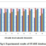Figure 4: Experimental results of STARE database Click here to view full figure

 

Conclusion

In this paper, we have developed an automated segmentation of blood vessel in retinal image system. The medical decision making system was designed with the Texture features and fuzzy logic based Support Vector Machine. The proposed approach comprises feature extraction and classification. The benefit of the system is to assist the physician to make the final decision without uncertainty. Our proposed vessel segmentation technique does not require any user intervention, and has consistent performance in both normal and abnormal images. The proposed blood vessel segmentation algorithm produces more than 96% of segmentation accuracy in both publically available DRIVE and STARE Database.

References

1. Doi, K.Computer-aided diagnosis in medical imaging: Historical review, current status and future potential.  Computerized Medical Imaging and Graphics, 31:198–211,2007.
2. .P.C.  Ronald, T.K.  Peng, A  Textbook of  Clinical Ophthalmology:  A  Practical Guide to  Disorders of   the  Eyes and  Their Management,  3rd  ed.,   World Scientific Publishing Company, Singapore, 2003.
3.  Sukkaew L, Makhanov B, Barman S, Panguthipong S (2008) Automatic tortuosity-based retinopathy of prematurity screening system. IEICE  transac- tions on information and systems 12.
4.   Koreen S, Gelman R, Martinez-Perez M (2007) Evaluation of a computer-based   system  for  plus  disease  diagnosis  in  retinopathy   of   prematurity. Ophthalmology 114(12): e59–e67.
5.   Niemeijer  M,  Xu  X,  Dumitrescu  A,  Gupta  P,  Ginneken  B,  et  al.  (2011) Automated measurement of the arteriolar-to-venular width ratio in digital color fundus photographs.  IEEE  Transactions  on  Medical Imaging 30(11): 1941–1950.
6.   Vickerman M, Keith P, Mckay T Vesgen (2009) 2d: Automated, user-interactive software for quantification and  mapping of angiogenic and  lymphangiogenic trees and networks. The Anatomical record 292.
7.    Leandro JJG, Cesar RM Jr. Blood vessels segmentation in retina: Preliminary assessment of the mathematical morphology & the wavelet transform techniques. Proceding on Computer Graphics and Image Processing 2001; 84-90
8.    Tolias YA, Panas SM. A fuzzy vessel tracking algorithm for retinal images based on fuzzy clustering. IEEE Trans Med Imaging 1998; 17:263-273.
9.   Zana, F, Kelin JC. Segmentation of vessel-like patterns using mathematical morphology and curvature evaluation. IEEE Trans on Image Process 2001; 10:1010-1019.
10.  Al-Rawi M, Karajeh H. Genetic algorithm matched filter optimization for automated detection of blood vessels from digital retinal images. Compute Methods Programs Boomed 2007; 87:248-253.
11.  T. Walter, P. Massin, A. Erginay, R. Ordonez, C. Jeulin, and J. C.Klein, “Automatic detection of microaneurysms in color fundus im- ages,” Med. Image Anal., vol. 11, pp. 555–566, 2007.
12.   Haralick, R. M., Shanmugam, K., & Dinstein, I. (1973). Textural features for image classification. IEEE Transactions on Systems, Man and Cybernetics SMC, 3(6), 610–621.
13.  Ondimu, S. N., & Murase, H. (2008). Effect of probability-distance based Markovian texture extraction on discrimination in biological imaging. Computers and Electronics in Agriculture, 63, 2–12
14. Idrissa M, Acheroy M: Texture classification using Gabor filters.Pattern Recognition Lett 23:1095–1102, 2002
15. Vapnik, V.N., 1982. Estimation of Dependences Based on Empirical Data, Secaucus. Springer-Verlag, New York.
16. Wang, T.Y. and H.M. Chiang, 2007. Fuzzy support vector machine for multi-class text categorization. Inform. Proc. Manage., 43: 914-929.
17.  C.F Lin, Wang S.E. ” Fuzzy support vector machines,”  IEEE Transactions on Neural Networks 13 , 464–471(2002).
18.  S. Haykin , Neural networks – A comprehensive foundation (second Ed.). Englewood Cliffs, NJ: Prentice-Hall. (1999).
19.  Y.L Huang, D.R Chen, “ Support vector machines in sonography. Application to decision making in the diagnosis of breast cancer,” . Journal of Clinical Imaging 29, 179–184, (2005).
20. Wen, Z., Z. Nancy and W. Ning, 2010. Sensitivity, specificity, accuracy, associated confidence interval and ROC analysis with practical SAS implementations. Proceeding of the SAS Conference. Baltimore, Maryland, pp: 9.

 

 

 

 

 

 

 

(Visited 1,160 times, 1 visits today)