P. Sunil Kumar and R. Harikumar

Research Scholar, Department of ECE Bannari Amman Institute of Technology India

DOI : https://dx.doi.org/10.13005/bpj/629

Abstract

Photoplethysmography (PPG) is used for the estimation of the blood flow of skin using an infrared light technique. It can measure parameters such as cardiac output, blood saturation level, blood pressure and oxygen saturation to a great extent. The greatest advantage of Photoplethysmography is that it is non-invasive in nature, has a low production and maintenance cost. For the early screening and detection of much body related pathologies PPG is the most developed and helpful tool nowadays. This paper analyses the PPG signals with respect to the parameters like Principal Component Analysis (PCA), Independent Component Analysis (ICA), Mutual Information (MI) and Entropy. PPG has also proved to be one of the most promising technologies for the early screening of heart related pathologies. This paper also analyses the PPG signals with respect to the parameters like Expectation Maximization (EM), Minimum Expectation Maximization (MEM) and Centre Tendency Moment (CTM).

Keywords

PPG; PCA; ICA; MI; Entropy EM; MEM; CTM

Download this article as: 

Copy the following to cite this article: Kumar P. S, Harikumar R. Performance Comparison of EM, MEM, CTM, PCA, ICA, Entropy and MI for Photoplethysmography Signals. Biomed Pharmacol J 2015;8(1)

Copy the following to cite this URL: Kumar P. S, Harikumar R. Performance Comparison of EM, MEM, CTM, PCA, ICA, Entropy and MI for Photoplethysmography Signals. Biomed Pharmacol J 2015;8(1). Available from: http://biomedpharmajournal.org/?p=1331

Introduction

The preliminary form of PPG technology generally requires only a few opto-electronic components namely, a light source which can illuminate the tissue (e.g. skin), and to measure the small variations in light intensity associated with respective changes in perfusion in the catchment volume a photo detector is used [1]. PPG is most often employed in a non-invasive manner and it specifically operates at near infrared wavelength [2]. The distinctive attribute of the waveform feature is the peripheral pulse, and it is causes to occur or operate at the same time and rate to each and every heartbeat. Despite its condition of being plain and uncomplicated the origins of the different components of the PPG signal are still not fully understood [3]. However, it is generally accepted that they can provide the most valuable and important information about the cardiovascular system. Photoplethysmography is somewhat related to but not equivalent to traditional plethysmography. The two basic modes are called as transmission mode PPG and reflectance mode PPG. In the case of the non-contact PPG, the drastic changes in the ambience which includes the surrounding light or the parameters like automatic brightness adjustment or even the software involved can have a vital effect on the baseline of the signal [4]. Apart from these factors, the physiologic parameters also have an effect on the baseline of the signal which includes the minor changes in the capillary density and the fluctuations in the venous volume.  PPG’s application is popularly available in the smart phone technology which is an important innovation in the contact reflectance PPG.  A high quality PPG signal can be easily recorded when the fingers are placed on the PPG which covers both the photo-light LED and also the camera lens [5]. Under normal conditions, because of the strongest modulation of the signal due to light absorption in the haemoglobin in the blood a wavelength in the near infrared is used. In this paper the Analysis of PPG Signals with respect to PCA, ICA, MI, Entropy, EM, MEM, CTM is done. The organization of paper is as follows, section 2 details the methodology of acquiring PPG signals from Pulse Oximeter and the significance of the parameters analyzed following the section 3 which explains the results and discussions.

Methodology

The PPG wave forms are obtained from four healthy subject using Dolphin Medical 2100 Pulse Oximeter in the Medical Electronics laboratory at Thiagarajar College of Engineering –Madurai. The experimental investigations confirm to the principles outlined in the declaration of Helsinki published in Br.Med.JL.1964, ii, 177. The PPG waveforms are recorded for five minutes durations and sampled at 100Hz through appropriate software coding. Then wave forms are added with Gaussian noise level of 1dB and 2dB levels to simulate a situation of motion artifacts.

Principal Component Analysis

Principal Component Analysis (PCA) is a dimensionality reduction technique that has been applied to many kinds of data. In fact, PCA is the optimal linear transform, i.e., for any choice for the number of dimensions, PCA returns the subspace that retains the highest variance [6].

PCA is a mathematical technique allows reducing the complex system of correlations in a smaller number of dimensions. χ being a table of P numeric variables (in   columns) describing N individuals (in lines), w propose to seek a representation of N individuals (signals) e1, e2,…en in a subspace of initial space. In other contexts, the K new variable has to defined, combination of P of initial space should be considered, which could make lossless possible information. These K variables will be called principal axes [6].

For N observations, we will have a matrix of N x P size which is given by

 

 

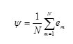
The average signal is defined by:

For each element the difference is given as follows

The computation of the covariance matrix can be done as follows:

 

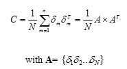
However, the determination of the Eigen vectors of covariance matrix will require an excessive calculation; the size of this matrix is (P x P). If υ_i is the eigen vector of AXA^T its eigen values are:

A^TAυ_i= μ υ_i

The Eigen vectors of C can be easily calculated as follows:

U_i=A υ_i                                                                                                                                                                                                                       

Ultimately the principal component of each signal e_i is given as follows

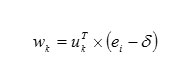
The vector w_k represents the new parameters completely de correlated and optimized for classification.

Independent Component Analysis

ICA is a variant of principal component analysis (PCA) in which the components are assumed to be mutually statistically independent instead of merely uncorrelated. It is a computational method for separating a multivariate signal into additive subcomponents supposing the mutual statistical independence of the non-Gaussian source signals [7]. A very versatile and simple application of ICA is the “cocktail party problem”, where for instance the sample data consisting of people talking simultaneously in a room can be separated from the underlying speech signals. Generally by assuming no time delays and echoes this problem could be easily simplified. It is vital to note that if Q sources are present, then at least Q observations are definitely required in order to get the original signals. This usually attributes to the square case, i.e., (A=D, where A gives the model’s dimension and D gives the input dimension of the data [7].

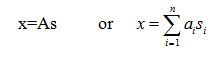
Independent Component Analysis describes a model for multivariate data describing large database of samples. The variables in the model are assumed non-Gaussian and mutually independent and they are called the independent components of the observed data. These are also called sources or factors. ICA is a powerful technique capable of finding the underlying factors or sources when the classic methods such as PCA fail completely.  Independent Component Analysis is used to uncover the independent source signals from a set of linear mixtures of the underlying sources. It is assumed that we observe n linear mixtures of x_1,…,x_n of  independent components are observed as shown in the following equation.

X_j=a_j1s₁+a_j1s₂+……..+a_jns_n,,      j=1,n

In this equation the variable x_j and the independent component s_i are random variables, x_j(t)and s_i(t) are samples of random variables. The variable and the independent component are also assumed to have zero mean reducing the problem to the model zero-mean and is given by the following equation.

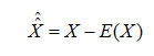
Let x and s be the random vector whose elements are x1,….,x_n and  s₁,….s_n respectively. Let A be the matrix containing the elements a_ij which is expressed as in Equation below

The above equation is called independent component analysis or ICA where only the measures variable x is available and the objective  is to determine both the matrix A and the independent components. The model is assumed to have independent and non-Gaussians components.  ICA decomposes multi dimensional data vector linearly to statistically independent components. ICA can be effectively used to remove artifacts and to decompose EEG recorded signals into different component signals originated from different sources. In the context of epilepsy detection, ICA is used to extract the independent sub components corresponding to epileptic seizure from the mixture of EEG signals.

Entropy

It is nothing but a measure of uncertainity of a particular random variable. The entropy H(X) for a particular discrete random variable X is defined as follows

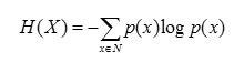
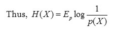
The entropy of X is also expressed as the expected value of log 1/p(X) where X is drawn according to probability mass function p(x).

 

Usually the above definition is related to the definition of entropy in thermodynamics.

Mutual Information

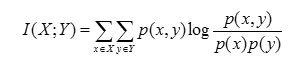
Mutual Information is nothing but the measure of the amount of information that one random variable contains about another random variable. By having the knowledge about the other random variable, the reduction in the uncertainity of one random variable can be easily done using mutual information. Two random variables X and Y are considered which has a joint probability mass function(x,y) and marginal probability mass function p(x) and p(y) [8].

The relative entropy between the joint distribution and the product distribution (i.e.) p(x) and p(y) is given as the mutual information I(X; Y) as is expressed mathematically as follows:

 

Expectation Maximization

The Expectation Maximization (EM) is often defined as a statistical technique for maximizing complex likelihoods and handling incomplete data problem [9]. EM algorithm generally consists of two steps namely:-

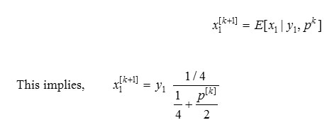
Expectation Step (E Step): Say for instance consider data  which has an estimate of the parameter and the observed data, the expected value is initially computed easily. For a given measurement and based on the current estimate of the parameter, the expected value of is computed as given below:

 

Maximization Step (M Step): From the expectation step, we use the data which was actually measured to determine the Maximum Likelihood estimate of the parameter [9]. The set of unit vectors is considered to be as Х. Considering x_i ∈ Х, the likelihood of Х is:

 

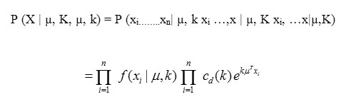
The log likelihood of the above equation can be written as:

L (Х|µ, k) = ln P (Х|µ, k) = n ln c_d (k) + k µ^Tr

where  r = ∑_ix_i

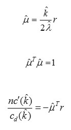
In order to obtain the likelihood parameters µ and κ, we will have to maximize equation (2.4) with the help of Lagrange operator λ. Then the modified equation can be written as:

L (µ, λ, κ, Х) = n ln c_d  (k) + k µ^Tr + λ (1-µ^T µ)

Derivating the above equation with respect to µ, λ & κ and equating these to zero will yield the parameter constraints as

 

In the Expectation step, the threshold data is first estimated when both the observed data and current estimate of the model parameters are given.  Conditional expectation is used to achieve this which clearly explains the choice of terminology. In the process of M – Step determination, the likelihood function is maximized under the assumption that the threshold data are known. The estimate of the missing data from the E – Step is used in lieu of the actual threshold data [9].

Modified Expectation Maximization (MEM) Algorithm

In this paper, a Maximum Likelihood (ML) approach which uses a modified Expectation Maximization (EM) algorithm for pattern optimization is used. Similar to the conventional EM algorithm, this algorithm alternated between the estimation of the complete log – likelihood function (E – Step) and the maximization of this estimate over values of the unknown parameters

(M – Step). Because of the difficulties in the evaluation of the ML function, modifications are made to the EM algorithm.

1. Find the initial values of the maximum likelihood parameters which are means covariance and mixing weights.
2. Assign each x_i to its nearest cluster centre c_k by Euclidean Distance (d)
3. In maximization step, use Maximization Q(θ θ’) .The likelihood function is written as:-

 

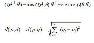
Repeat iterations and do not stop the loop until ||θⁱ⁺¹– θⁱ|| becomes small enough.

The algorithm ends when the difference between the log likelihood for the previous iteration and current iteration fulfills the tolerance level. The method of maximum likelihood corresponds for many well – known statistical estimation methods. For instance , one may be very interested to learn about the heights of adult female giraffes in a particular zoo, but it might be unable because of time and permission constraints, to measure the height of each and every single giraffe in that population. If the heights are assumed to be normally Gaussian distributed with some unknown mean and variance, then the mean and variance can be estimated mostly with Maximization Likelihood Equalization (MLE) by just knowing the heights of some of the samples of the overall population.

Centre Tendency Mode

Central Tendency Measure (CTM) which is used to quantify the degree of variability in the third order differential plots as shown in the Figures 2.1 and 2.2. The CTM is computed by selecting a circular region of radius ‘r’ and dividing by the total number of points [10].  Let t=total number of points and R is the radius of the central area, then

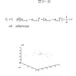Figure 2.1: CTM Plot for the Clean PPG Signal Click here to View figure

 

 

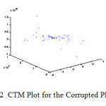Figure 2.2:  CTM Plot for the Corrupted PPG Signal Click here to View figure

 

Results and Discussion

The results and discussion have been clearly tabulated as shown in table 3.1 and table 3.2. The PPG signals have been analyzed thoroughly for the both the noise corrupted PPG signal and the noise free PPG signal. The performance evaluation parameters like the PCA, ICA, Entropy and MI is discussed clearly in table 3.1.

Table 3.1: Parameters analyzed for the PPG signal and the corrupted PPG signal

PARAMETERS ANALYZED	PPG SIGNAL	CORRUPTED PPG SIGNAL
PCA	0.9977	0.9774
ICA	0.3501	0.2035
Entropy	0.2138	0.1978
Mutual Information (MI)	0.0628	0.0016
Hurst Exponent for MI	0.42	0.32

 

From the above Table 3.1, it is clear that the noise free PPG signal the PCA yields a slightly higher value than for the corrupted PPG Signal. The ICA value is also comparatively higher for the Clean PPG Signal when compared to that of the Corrupted PPG Signal. The Entropy for the Clean PPG Signal is higher with a value of about 0.2138 when compared to that of the noisy PPG Signal which has a value of about 0.1978. The Mutual Information value is very low for the corrupted PPG Signal as of 0.0016 while it is slightly higher for the clean PPG Signal as of 0.0628. The Hurst Exponent Values taken for the Mutual Information yields a value below 0.5 for the both the clean and corrupted signal thereby it shows that both the signals are rhythmic and non-linear in nature. Future work involves the statistical analysis of PPG Signals and then using suitable classifiers, the work is planned to be extended for the classification of any diseases in human mankind.

The performance evaluation parameters like the Expectation Maximization, Modified Expectation Maximization and Centre Tendency Moment is discussed clearly in table 3.2 The PPG signals have been analyzed thoroughly for the both the noise corrupted PPG signal and the noise free PPG signal.

Table 3.2: Parameters analyzed for the PPG signal and the corrupted PPG signal

PARAMETERS ANALYZED	PPG SIGNAL	CORRUPTED PPG SIGNAL
Expectation Maximization	0.0478	0.0473
Modified Expectation Maximization	Mean=8.3407	Mean=0.5590
	Variance=1.8682	Variance=0.2793
Centre Tendency Moment	0.0417	0.0794
	No. of points inside=46	No. of points inside=5
	No. of points outside=2	No. of points outside=58

 

From the above Table 3.2, it is clear that the noise free PPG signals has a slightly greater Expectation Maximization Value when compared to that of the Corrupted PPG Signal. Also if we consider the Modified Expectation Maximization Algorithm for the Clean PPG Signal, the Mean is about 8.34 and the Variance is about 1.86 and if we consider the Modified Expectation Maximization Algorithm for the Corrupted PPG Signal, then the Mean produced is very less about 0.55 and the Variance produced also is less and is about 0.27. The Centre Tendency Moment is less and optimum for the Clean PPG Signal and it is higher for the Corrupted PPG Signal. Future work involves the statistical analysis of PPG Signals and then using suitable classifiers, the work is planned to be extended for the classification of any diseases in human mankind.

References 

1. Allen J , “The measurement and analysis of multi-site photoplethysmographic pulse waveforms in health and arterial disease” PhD Thesis Newcastle University, 2002
2. Allen J and Murray A , “Effects of filtering on multi-site photoplethysmography pulse waveform characteristics” IEEE Comput. Cardiol. 31,2004,485–8
3. Allen J, et al, “ Photoplethysmography assessments in cardiovascular disease”, Control 39 ,2006, 80–3
4. Azabji Kenfack M, Lador F, Licker M, Moia C, Tam E, Capelli C, Morel D and Ferretti G Cardiac output by Modelflow method from intra-arterial and fingertip pulse pressure profiles Sci. 106 ,2004, 365–9
5. Bhattacharya J, Kanjilal P P and Muralidhar V Analysis and characterization of photo-plethysmographic signal IEEE BME 48 , 2001,5–11
6. Harikumar R and Vijayakumar T, “Wavelets and Morphological Operators Based Classification of Epilepsy Risk Levels,” Mathematical Problems in Engineering, vol. 2014, Article ID 813197, 13 pages, 2014. doi:10.1155/2014/813197.
7. Harikumar R and Vijayakumar T, Performance Analysis of Elman- Chaotic Optimization Model for Fuzzy Based Epilepsy Risk level Classification from EEG Signals, International Journal on smart sensing and Intelligent Systems Vol 2 no: 4 Dec2009 ,pp 612-635.

(Visited 449 times, 1 visits today)