
Manuscript accepted on :
Published online on: 26-12-2015
Plagiarism Check: Yes
Ayush Dogra and Parvinder Bhalla
Department of ECE, Maharishi Markandeshwar University, Mullana, Ambala, India.
DOI : https://dx.doi.org/10.13005/bpj/545
Abstract
Many significant images contains some extent of noise, that is unexplained variation in data disturbances in image intensity which are either uninterpretable or out of interest. Image analysis is often simplified if this unwanted noise is filtered. For this image simplification, filtering in frequency domain is done. In this paper we will demonstrate the image sharpening by Gaussian & Butterworth high pass filter and jot some points revealing their differences.
Keywords
Gaussian; Butterworth; image analysis; frequency domain
Download this article as:| Copy the following to cite this article: Dogra A, Bhalla P. Image Sharpening By Gaussian And Butterworth High Pass Filter. Biomed Pharmacol J 2014;7(2) |
| Copy the following to cite this URL: Dogra A, Bhalla P. Image Sharpening By Gaussian And Butterworth High Pass Filter. Biomed Pharmacol J 2014;7(2). Available from: http://biomedpharmajournal.org/?p=3274 |
Introduction
Filter out unwanted frequencies from the image is called filtering. The objective of image filtering is to process the image so that the result is more suitable then the original image for a specific applications. Image filtering refers to a process that removes the noise, improves the digital image for varied application. The basic steps in frequency domain filtering are shown in figure 1.
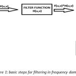 |
Figure 1: basic steps for filtering in frequency domain |
Fourier transform will reflect the frequencies of periodic parts of the image. By applying the inverse Fourier transform the undesired or unwanted frequencies can be removed and this is called masking or filtering. A filter is a matrix, and components of the filters usually vary from 0 to 1. If the component is 1, then the frequency is allowed to pass, if the component is 0 the frequency is tossed out.
A large variety of image processing task can be implemented using various filters. A filter that attenuates high frequencies while passing low frequencies is called low pass filter. Low pass filter are usually used for smoothing. Whereas, a filter that do not affect high frequencies is called high pass filter. High pass filters are usually used for sharpening. Furthermore, band pass (band reject filter) work on specific frequencies bands. Notch filters work on specific frequencies. Low pass, high pass & band reject filters are often called ideal filters, though they have jumps as shown in figure2.
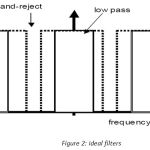 |
Figure 2: ideal filters |
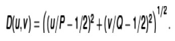
An ideal filter has the property that all frequencies above (or below) a cut off frequency Do are set to zero[2]
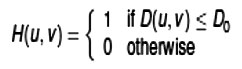
Where
Gaussianfilter
Definition
The one-dimensional Gaussian filter has an impulse response given by
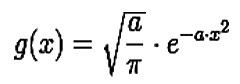
And the frequency response is given by
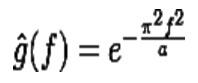
With ƒ the ordinary frequency. These equations can also be expressed with the standard deviation as parameter
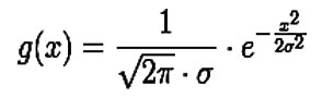
And the frequency response is given by
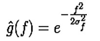
By writing as a function of with the two equations for and as a function of with the two equations for it can be shown that the product of the standard deviation and the standard deviation in the frequency domain is given by
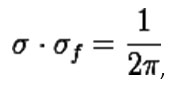
Where the standard deviations are expressed in their physical units, e.g. in the case of time and frequency in seconds and Hertz.
In two dimensions, it is the product of two such Gaussians, one per direction:
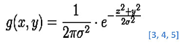
Wherex is the distance from the origin in the horizontal axis, y is the distance from the origin in the vertical axis, and σ is the standard deviation of the Gaussian distribution.
Gaussian Low Pass And High Pass Filter In Frequency Domain[1, 2, 7]
In the case of Gaussian filtering, the frequency coefficients are not cut abruptly, but smoother cut off process is used instead. Thus also takes advantage of the fact that the DFT of a Gaussian function is also a Gaussian function shown in figure 6,7,8,9. The Gaussian low pass filter attenuates frequency components that are further away from the centre (W/2, H/2), A~1/σWhere σ is standard deviation of the equivalent spatial domain Gaussian filter.
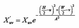
The Gaussian high pass filter attenuates frequency components that are near to the image center (W/2, H/2);
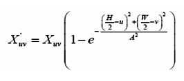
Figure 3, 4, 5 shows the result of Gaussian filter. Ringing (wave) effect is avoided in the Gaussian filter.
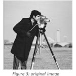 |
Figure 3: original image
|
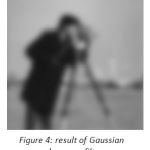 |
Figure 4: result of Gaussian
|
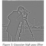 |
Figure 5: Gaussian high pass filter low pass filter |
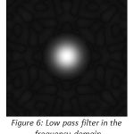 |
Figure 6: Low pass filter in the frequency domain |
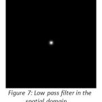 |
Figure 7: Low pass filter in the spatial domain
|
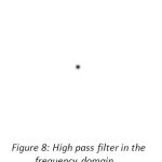 |
Figure 8:High pass filter in the frequency domain |
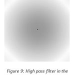 |
Figure 9: High pass filter in the Spatial domain |
Butterworth Filter
Definition
Another version of smoothing/ sharpening filters are the Butterworth filter. A Butterworth filter of order n and cutoff frequency D0 is defined as [2, 7]
An advantage with the Butterworth filter is that we can control the sharpness of the filter with the order.
Butterworth Low Pass Filter
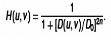
A Butterworth low pass filter keeps frequencies inside radius D0 and discard value outside it introduces a gradual transition from 1 to 0 to reduce ringing artifacts. The transfer function of a Butterworth low pass filter (BLPF) of order n, and with cutoff frequency at distance D0 from the origin, is defined as [2, 7]
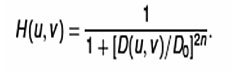
Figure 11, 12, 13, 14, 15 show the result of applying Butterworth low pass filter to figure 10, with n = 2 and Do equal to 10,30,60,160 and 460. Therefore notice a smooth transition in blurring as a function of increasing cutoff frequency. No ringing is visible in any of the images processed with this particular BLPF.
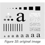 |
Figure 10: original image
|
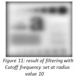 |
Figure 11: result of filtering with Cut off frequency set at radius value 10
|
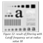 |
Figure 12: result of filtering with Cut off frequency set at radius value 30
|
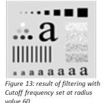 |
Figure 13: result of filtering with Cutoff frequency set at radius value 60 |
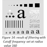 |
Figure 14: result of filtering with Cutoff frequency set at radius value 160
|
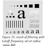 |
Figure 15: result of filtering with Cutoff frequency set at radius value 460 |
Butterworth High Pass Filter[1, 2, 7]
A Butterworth high pass filter keeps frequencies outside radius D0 and discards values inside. It has a gradual transition from 0 to 1 to reduce ringing artifacts. A Butterworth highpass filter (BHPF) of order n and cutoff frequency D0 is defined as
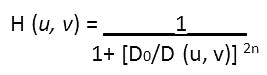
Figure 17, 18,19 shows the result of applying Butterworth high pass filter on figure 16,with n = 2, and Do equal to 30,60 and 160. These results are much smoother. The boundaries are much less distorted, even for the smallest value of cutoff frequency. The transition into higher values of cutoff frequencies is much smoother with the BHPF.
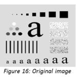 |
Figure 16: Original image |
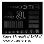 |
Figure 17: result of BHPF of order 2 with D0 = 30 |
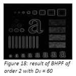 |
Figure 18: result of BHPF of order 2 with D0 = 60 |
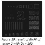 |
Figure 19: result of BHPF of order 2 with D0 = 160 |
3d Perspective Plot Of Filter’s Transfer Function [2]
The ideal low pass filter is radially symmetric about the origin, which means that the filter is completely defined by radial cross section as shown in figure 20. Unlike the ILPF, the BLPF transfer function does not have a sharp discontinuity that gives a clear cutoff between passed and filtered
Frequencies as depicted in figure 21. For filter with smooth transfer functions, defining a cutoff frequency locus at points for which H(u, v) is down to a certain fraction of its maximum value is customary. Perspective 3D plot of GLPF is shown in figure 22. Unlike the ILPF, GLPF transfer function also does not have sharp discontinuity but it is much smoother than BLPF. Butterworth filter represents the transition between the sharpness of the ideal filter and broad smoothness of the Gaussian filter. Figure 23, 24, and 25 shows the perspective 3D plots of IHPF, BHPF and GHPF.
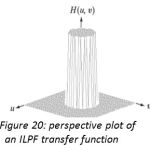 |
Figure 20: perspective plot of an ILPF transfer function
|
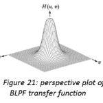 |
Figure 21: perspective plot of BLPF transfer function
|
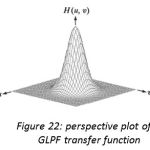 |
Figure 22: perspective plot of GLPF transfer function
|
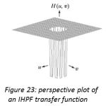 |
Figure 23: perspective plot of an IHPF transfer function
|
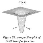 |
Figure 24: perspective plot of BHPF transfer function
|
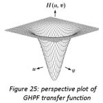 |
Figure 25: perspective plot of GHPF transfer function |
Image Sharpening With Gaussian and Butterworth High Pass Filter
High pass filter give emphasis to the higher frequencies in the image. The high pass image is then added to the original image so as to obtain a sharper image.[6] It may be interesting to experiment with width and frequency threshold of the Butterworth or the Gaussian high pass filters and it will really interesting to compare the sharpening which is done in frequency domain and can compare it with the sharpening done in spatial domain. We will only demonstrate the image sharpening using Gaussian and Butterworth high pass filter taking Do=100,n=4(where Do is cutoff frequency, n is the order of the filter). Figure 26 is the CT image, figure 27 depicts the FFT of the image, and figure 28shows the Butterworth high pass filter of FFT image. Figure 29 shows the Gaussian high pass filter of FFT image. Similar examples are shown with MRI image in figure 30. Figure 31, 32, 33 shows FFT of image, Butterworth high pass filter of FFT image, Gaussian high pass filter of FFT image. Now the resultant sharpened images of CT and MRI image are shown in figure 34,35,36,37. Now these sharpened images can be used in various image processing tasks, like edge detection and ridge detection.
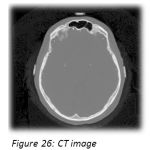 |
Figure 26: CT image |
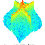 |
Figure 27: FFT of CT image |
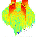 |
Figure 28: BHPF of FFT image |
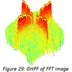 |
Figure 29: GHPF of FFT image |
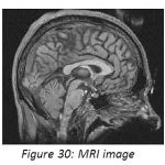 |
Figure 30: MRI image
|
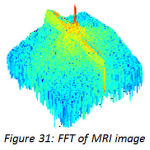 |
Figure 31: FFT of MRI image
|
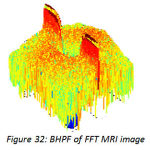 |
Figure 32:BHPF of FFT MRI image |
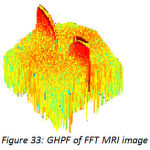 |
Figure 33: GHPF of FFT MRI image
|
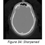 |
Figure 34: Sharpened image by BHPF |
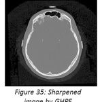 |
Figure 35: Sharpened image by GHPF |
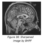 |
Figure 36: Sharpened image by BHPF
|
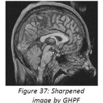 |
Figure 37: Sharpened image by GHPF
|
Conclusion and Result
We use Do=100,n=4 & uses Gaussian and Butterworth high pass filter . High pass filter give emphasis on the high frequencies in the image. The difference between Butterworth and Gaussian filters is that the former is much sharper than latter. The resultant images by BHPF is much sharper than GHPF ,while analysis the FFT of CT and MRI image, one sharp spike is concentrated in the middle. By applying BHPF & GHPF on the images, we find drastically change in the color intensities of high pass filter of FFT images. The split edges are elongated and wider in BHPF case than GHPF. But in GHPF case the split edges are sharper. These elongated split edges in BHPF leads to sharper image than GHPF.
References
- Umbaugh Scot E, Computer Vision and Image Processing, Prentice Hall, NJ, 1988, ISBN 0-13-264599-8
- R.C.Gonzales, R.E.Woods, Digital Image Processing, 2-nd Edition, Prentice Hall, 2002
- R.A. Haddad and A.N. Akansu, “A Class of Fast Gaussian Binomial Filters for Speech and Image Processing,” IEEE Transactions on Acoustics, Speech and Signal Processing, vol. 39, pp 723-727, March 1991.
- Shapiro, L. G. & Stockman, G. C: “Computer Vision”, page 137, 150. Prentence Hall, 2001
- Mark S. Nixon and Alberto S. Aguado. Feature Extraction and Image Processing. Academic Press, 2008, p. 88.
- Yusuf, Nijad, Sara Tedmory “Exploiting hybrid methods for enhancing digital X-ray images”. The International Arab Journal of Information Technology, Vol. 10, No.1, January 2013.
- Gonzales R., Woods R., and Eddins S., Digital Image Processing Using Matlab, 2nd Edition, Prentice Hall, USA,

