G. Hari Krishnan¹, Anima Nanda¹ and Ananda Natarajan R²

¹Department of Biomedical Engineering, Sathyabama University, Chennai, India.

²Department of Electronic and Instrumentation, Pondicherry Engineering College, Pondicherry, India.

DOI : https://dx.doi.org/10.13005/bpj/476

Abstract

Synovial fluid generally present in the joint region for the purpose of lubricant as a major task. During arthritis disease affected condition the density of synovial fluid varies as a function of time in case of osteoarthritis and as a function of disease condition in case of rheumatoid arthritis. By measuring the variation in density of synovial fluid arthritis diseases can be diagnosed. In this paper an non invasive method has been adopted for measurement of synovial fluid density change using electrical bio-impedance concept. Electrical Bio-Impedance is the measure of opposition given by the tissue for applied electrical signal. The Bio-impedance values are measured in terms of voltage drop across the joint tissue region as tissue can be represented as resistance and capacitive reactance. These resistance and reactance varies from normal person to Arthritis patient for a fixed frequency and voltage. Hardware section made using signal generator circuit with variable frequency and variable voltage provision. To measure the voltage drop using non invasive method four electrodes has been utilized for given electrical signal and acquiring the response.

Keywords

Synovial fluid density; Arthritis; Electrical bio-impedance; Non invasive diagnosis; Electrodes

Download this article as: 

Copy the following to cite this article: Krishnan G. H, Nanda A, Natarajan A. R. Synovial Fluid Density Measurement for Diagnosis of Arthritis. Biomed Pharmacol J 2014;7(1)

Copy the following to cite this URL: Krishnan G. H, Nanda A, Natarajan A. R. Synovial Fluid Density Measurement for Diagnosis of Arthritis. Biomed Pharmacol J 2014;7(1). Available from: http://biomedpharmajournal.org/?p=2920

Introduction

Arthritis, human joint disorder was analysed generally by invasive methods, blood test, Pathology, X-ray, MRI, Ultrasound, CT and Synovial fluid test. Based on the sign and symptoms obtained during initial diagnosis the doctor advices to go for any one of the above test [2, 3]. The diagnosis ends with basic blood test and x-ray for initial stage patients. For advance stage diagnosis the patient needs to go for MRI, Synovial Fluid test or ultrasound test. During these conventional methods either blood has to be taken out or body fluid has to be collected from region of interest by undergoing minor surgery [4, 5].  From the advancement in medical diagnosis technology as optical sensing and bio-impedance makes the possibility of non invasive diagnosis. The Bio-impedance spectroscopy has been used to monitor body fluid volume, Water content in body, Cardiac output etc., with non invasive system. The potential problems of the affected tissue can be identified by measuring impedance of a set of tissues using invasive method [1, 6].

Bio-impedance spectroscopy diagnosis system design was made of constant current source as an essential part. Current source are widely obtained from voltage to current converter and Howland current source [9].  Bio-impedance analysis uses mathematical analogues and complex equations to find the resistance of body fluid. The resistance measurement varies as input frequency varies from zero to infinity [10]. During implementation of bio-impedance based non invasive method for diagnosis of arthritis the diagnosed output value obtained on the skin surface near the joint region varies as the function of input voltage and frequency. This paper analyse the effect of input frequency and input voltage variations on output reading.

Experiment And Observation

The non invasive system for diagnosis of arthritis was designed using signal generator with the provision of varying the frequency ranging from 10 KHz to 500 KHz and varying the voltage ranging from 0 Volts to 8 Volts. To have non invasive contact with joint region four electrodes have been used. The purpose of four electrodes is to give electrical signal in to the tissue region and also to collect the response of the tissue to the applied electrical signals [7, 8]. The passage of electrical signal through tissue was opposed by the electrical property of the tissues called electrical bio-impedance. This opposition given by the tissue to the applied signal has been measured in terms of voltage drop. The obtain voltage signal was processed using data acquisition unit and display using voltage display unit as shown in figure 1. These resistance and reactance varies from normal person to Arthritis patient for a fixed frequency and voltage. If input voltage or frequency was varied the measured voltage drop in terms of bio-impedance varies.

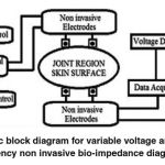Figure 1: Basic block diagram for variable voltage and variable frequency non invasive bio-impedance diagnosis   Click here to View figure

 

The readings which were obtained from the joint region using non invasive electrodes were separated in to two tabulations. The first tabulation contains output voltage values for constant input frequency of 200 KHz as shown in table 1. Similarly second tabulation contains voltage values for constant input voltage of 8 Volts as shown in table 2. From table 1 we observe that for the fixed input frequency 200 KHz the output voltage varies as a function of input voltages. By varying input voltage from 1 Volts to 8 Volts we observed that output voltage varies from 0.08 Volts to 3.70 Volts.

Table 1: Voltage values obtained in terms of bio-impedance for fixed frequency and variable input voltage

Output voltage in Volts variation for Constant Frequency = 200 KHz
V1 = 1 Volts	V2 = 3 Volts	V3 = 6 Volts	V4 = 8 Volts
0.14	0.25	1.00	1.80
0.14	0.27	1.28	2.17
0.19	0.29	1.34	2.32
0.21	0.33	1.39	2.45
0.25	0.38	1.48	2.75
0.30	0.42	1.62	2.98
0.34	0.47	1.79	3.08
0.38	0.51	1.89	3.28
0.41	0.56	2.18	3.46
0.45	0.60	2.50	3.70

 

In the tabulation the output voltage readings were arranged in age order so we observe that the older the age higher was the voltage drop for same value of input voltage.  Similarly from table 2 we observe that for the fixed input voltage of 8 V the output voltage varies as a function of input frequency. By varying input frequency from 50 KHz to 200 KHz we observed that output voltage varies from 0.14 Volts to 3.70 Volts.

Table 2: Voltage values obtained in terms of bio-impedance for fixed voltage and variable input frequency

Output voltage in Volts variation for Constant Input Voltage = 8 Volts
50 KHz	100 KHz	150 KHz	200 KHz
0.08	0.13	0.98	1.82
0.11	0.19	1.06	2.16
0.13	0.21	1.12	2.3
0.14	0.23	1.21	2.42
0.15	0.25	1.26	2.75
0.19	0.27	1.32	2.98
0.22	0.31	1.37	3.08
0.25	0.33	1.43	3.26
0.31	0.4	1.54	3.46
0.26	0.43	1.6	3.73

 

Results and Discussion

Using the values in tabulations two graphs was plotted. The voltage variation based on age for different input voltage variations has been shown in figure 2. Output voltage varies as a function on age as well as input voltage variation has been clearly observed from the four different curves. For constant frequency of 200 KHz the out voltage oscillates from 0.14 Volts to 3.7 Volts. The voltage variation based on age for different input frequency changes has been shown in figure 3.

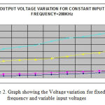Figure 2: Graph showing the Voltage variation for fixed frequency and variable input voltages   Click here to View figure

 

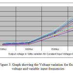Figure 3: Graph showing the Voltage variation for fixed voltage and variable input frequencies   Click here to View figure

 

Output voltage varies as a function on age as well as input frequency variation has been clearly observed from the plotted curves. For constant voltage of 8 Volts the out voltage oscillates from 0.08 Volts to 3.73 Volts. From the two graphs we can observe that the output voltage varies as age varies. High voltage drop for persons with older age and low voltage drop for person with young age irrespective of the input voltage and frequency variation.

Conclusion

The synovial fluid density changes have been observed in terms of voltage drop. Also the voltage drop variation for variation in input frequency and input voltage has been observed. The current study implements analyses of the impact of input voltage and frequency variation during bio-impedance based diagnosis. These resistance and reactance varies from normal person to Arthritis patient for a fixed frequency and voltage. If input voltage or frequency was varied the measured voltage drop in terms of bio-impedance varies. In this paper the effect of input frequency and voltage on output measurement has been analysed with circuit made using signal generator circuit with variable frequency and variable voltage provision.

References

1. Ibrahim, N. A. Ismail, M. N. Taib, W. A. B. Wan Abas, S. Sulaiman, and C. C. Guan, “Assessment of haematocrit status using bioelectrical impedance analysis in dengue patients”, IFAC Modelling and Control in Biomedical Systems, Melbourne, Australia, 2003.
2. Hari Krishnan, R. Ananda Natarajan and Anima Nanda. “Variable Frequency Signal Generator for Non Invasive Bio-impedance Diagnosis”. Indian Stream Research Journal, Volume 4, Issue 1, 2014.
3. Hari Krishnan, R. Ananda Natarajan and Anima Nanda. “Chronic, Systemic Inflammatory Disorder Development Stages Diagnosis Using Image Analysis Tools” ICDMSCT’13 on Oct 25 & 26, 2013, SASTRA University.
4. Hari Krishnan, R. Ananda Natarajan and Anima Nanda. “Detection of Synovial Fluid Variation and Its Impact on Joint Diseases Diagnosis” in INCAM-2013, IIT Madras on 4-6 July 2013.
5. Houman Mirzaalian Dastjerdi, Ramin Soltanzadeh, Hossein Rabbani. “Designing and Implementing Bioimpedance Spectroscopy Device by Measuring Impedance in a Mouse Tissue. Journal of Medical Signals and Sensors”, Vol 3, Issue 3, Jul-Sep 2013.
6. Neves E. B., Pino A.V., R. M. V. R. Almeida and Souza M. N.,. “Objective Assessment of Knee Osteroarthritis in Parachuters by Bioimpedance Spectroscopy”. 30^th Annual International IEEE EMBS conference, 2008, Pages: 5620-5623.
7. Suhas S. Gajre, Sneh Anand, U. Singh, Rajendra K. Saxena. “Novel Method of Using Dynamic Electrical Impedance Signals for Noninvasive Diagnosis of Knee Osteoarthritis”, Proceedings of the 28^th EMBS Annual International conference, 2006, Pages: 2207 – 2210.
8. Zlochiver, M. Arad, M.M. Radai, D. Barak-Shinar, H. Krief, T. Engelman, R. Ben-Yehuda, A. Adunsky, S. Abboud. “A portable bio-impedance system for monitoring lung resistivity”. Medical Engineering & Physics 29 (2007) 93–100.
9. Shekh Md Mahmudul Islam*, Mohammad Anisur Rahman Reza and Md Adnan Kiber. “Performance of Multi-Frequency voltage to current converters for bioimpedance spectroscopy”. Bangladesh Journal of Medical Physics Vol. 5, No.1, 2012.
10. Ursula G. Kyle, Ingvar Bosaeus, Antonio D. De Lorenzo, Paul Deurenberg, Marinos Elia, Jos!e Manuel G!omez, Berit Lilienthal Heitmann, Luisa Kent-Smith, Jean-Claude Melchior, Matthias Pirlich, Hermann Scharfetter, Annemie M.W.J. Schols, Claude Pichard. “Bioelectrical impedance analysisFpart I: review of principles and methods Composition of the ESPEN Working Group”. Elsevier, Clinical Nutrition (2004) 23, 1226–1243.

(Visited 1,419 times, 1 visits today)