Janar J. Yermekbayeva

L. N. Gumilyov Eurasian National University, Faculty of Physics and Technical Sciences, Department System Analyses and Control, 2 Mirzoyan Street, Astana - 010 008, Kazakhstan.

DOI : https://dx.doi.org/10.13005/bpj/417

Abstract

In this paper, we present a new mathematical analysis that models the growth and control of tumors in living tissue. In these models, we use the D-factor, a fold form from catastrophe theory, to impose control on tumor growth. By adjusting parameters, the models exhibit stationary states at which the immune system is stabilized and the number of tumor cells is either driven to zero or remains constant.

Keywords

Regulation of immune system; Control system; Robust stability; Lyapunov function; Compensatory effect; D-factor; Structurally steady mappings; Bifurcation values

Download this article as: 

Copy the following to cite this article: Yermekbayeva J. J. Structurally Steady Control of Tumor Cell Populations. Biomed Pharmacol J 2013;6(2)

Copy the following to cite this URL: Yermekbayeva J. J. Structurally Steady Control of Tumor Cell Populations. Biomed Pharmacol J 2013;6(2). Available from: http://biomedpharmajournal.org/?p=2729

Introduction

Modern medicine is providing reliable approaches for screening, diagnosis, treatment, prevention, and early intervention of cancer. Fortunately, current research levels are high enough to identify many cancer types as curable and studies are underway to find those cures.

In this work, we study mathematical models for tumor growth. Some previous studies have developed mathematical models for biological immune systems. For example, Adimya and Crauste considered a nonlinear mathematical model of hematopoietic stem cell dynamics in which proliferation and apoptosis are controlled by growth factor concentrations [1].

Structured models were found by Roeder et al. [2] to consistently explain a broad variety of phenomena in patients with chronic myeloid leukemia. Furthermore, Kim et al. [3, 4] developed a model for describing the dynamics during the treatment of chronic myelogenous leukemia. This model is intended to replace the recent agent-based model.

By changing the initial susceptible population after each epidemic generation, models developed by Roeder et al. [5] incorporate the effects of vaccination.

In this work, we model tumor growth by considering interactions between tumor cells and cells that resist cancer growth, that is, cells that regulate antitumor activity. The latter can be viewed as a control system applied to tumors, and the creation of models that combine control laws with a class of structurally steady mappings constitutes a new approach to cancer study. The work may be important for both its practical applications and its theoretical novelty.

To develop and test new models in the theory of control in immunology, we apply classical and modern theories of control, theoretical and applied methods in the study of dynamic systems, modern catastrophe theory and its application to population models, and Lyapunov stability theory.

We view cancer as uncontrolled proliferation of tumor cells in an organism. Our task is to suppress outbreaks and stabilize the organism (through the influence of a vaccine) when outbreaks do occur.

Mathematical Models

To track the growth of tumor and tumor-resistant cell populations, we start with a relatively simple model (§ 2.1). Then we add terms to account for the control of tumor growth (§ 2.2) and determine the stability of that extended model (§ 2.3). Then we extend the model further to account for the suppression of the boomerang effect (§ 2.4).

Initial Model

To model cell populations, including their interactions and influence, we start with two dynamical variables: the concentration of tumor cells and the concentration of cells that have specific resistance to tumor growth. Cells with natural resistance have some level of activity, which is included in the model as a parameter.

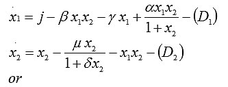
In particular, the temporal evolution of the two concentrations is modeled by these two differential equations [6]:

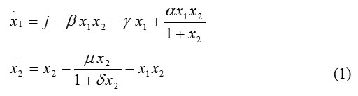
Here x₁ is the concentration of free cells (effector cells), x₂ is the concentration of tumor cells, j is the growth rate of effector cells, bx₁x₂ is the death rate of effector cells due to their interactions with tumor cells, x₁x₂ is the death rate of tumor cells due to their interactions with effector cells, a controls the growth rate of effector cells due to interactions with tumor cells, d controls the growth rate of tumor cells, g controls the natural death rate of effector cells, and m controls the natural death rate of tumor cells. Thus, our model is a system of two differential equations involving six parameters.

The phase portrait [7, 8] for system (1) is shown in Fig. 1. The stationary points of the model are determined from the conditions x₁ = 0 and x₂ = 0. Therefore, from (1), model 1 has three equilibrium states: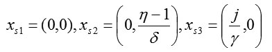

These are marked by the filled circles in Fig. 1.

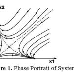Figure 1: Phase Portrait of System (1).   Click here to View figure

 

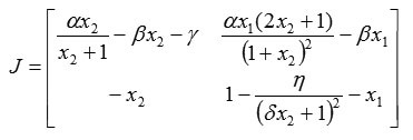
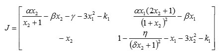
Note that the Jacobi matrix of system (1) is

Adding a Control Law to the Initial Model

To promote the stabilization of an organism in a predictable manner, we present a new method for controlling cell populations through interactions between effector and tumor cells. We call this approach a “compensatory effect.”

To model system (1), we add a synchronic controlling D-factor, which is a function of structurally steady mappings known as a “fold catastrophe.” One of the most important points in catastrophe theory is the behavior of smooth functions that depend on a parameter. The D-factor used here represents a fold form (one of the 7 forms of catastrophe theory) [9, 10]. Then model (1) becomes

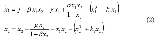
Negative values indicate a specific influence on the organism. The controlling parameter can be thought of as the influence of the therapy (vaccination) being received.

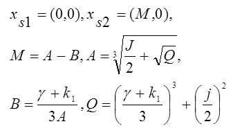
Stationary points are determined from the conditions , and therefore, system (2) has these equilibrium states:

The phase portrait of system (2) is shown in Fig 2.

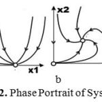Figure 2: Phase Portrait of System (2).   Click here to View figure

 

The Jacobi matrix of system (2) is

Region of Stability for the Extended Model

We now determine the conditions at which the system of nonlinear equations (2) exhibits stability. To this end, we construct the Lyapunov function. We also use the central Morse theorem with fold catastrophe from the classification of Thom’s theorem.

Stability is a fundamental notion in the qualitative theory of differential equations and is essential for many applications. In turn, Lyapunov functions are a basic instrument for studying stability; however, there is no universal method for constructing Lyapunov functions. Nevertheless, in some special cases, a function can be constructed by applying special techniques [11, 12].

We construct the Lyapunov function for system (2) and then use geometric interpretation to find the region of stability. The geometric identification of stable states reduces to creating a family of closed surfaces that surround the zero equilibrium of coordinates. The system state moves across contour curves; that is, each integrated curve can cross each of these surfaces, as illustrated in Fig. 3.

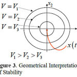Figure 3: Geometrical Interpretation of Stability   Click here to View figure

 

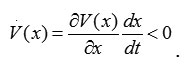
To apply the geometric interpretation, we must find the Lyapunov function, which is a positive definite state function V(x) > 0 whose time derivative is locally negative definite  < 0 or

It is known that this system can be described by these dynamical equations:

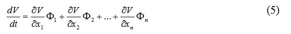
It is also known that the time derivative of the corresponding Lyapunov function has the form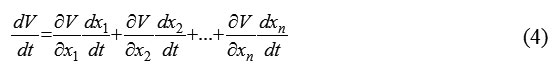

or

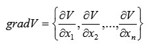
The gradient of a function  is a vector defined by

We can introduce a vector  with projections corresponding to (3), namely

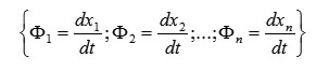
The vector  is a velocity vector of a point M, as depicted in Fig 4.

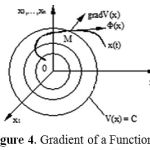Figure 4: Gradient of a Function.   Click here to View figure

 

According to (4) and (5), we have

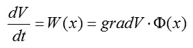
where.The time derivative of the Lyapunov function is a scalar product of the gradient and the phase velocity vector. Note that in Fig. 4, the vector is perpendicular to the surface  and is in the direction of the maximum increase in .

Now, we construct the vector function

whose gradient has a magnitude equal to the absolute value of the velocity vector for system (2) and whose direction is opposite to that of the velocity vector. For system (2), we form components of the gradient-vector Lyapunov function and find

and

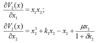
Then the full derivative of the Lyapunov function is

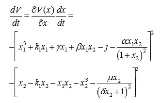
This expression shows that dV/dt < 0.

To find the integral components, we integrate

only over  and integrate

only over . We also integrate

and

first over  and then over . Therefore, we have [13]

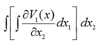
and

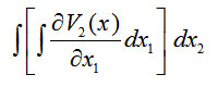
We find

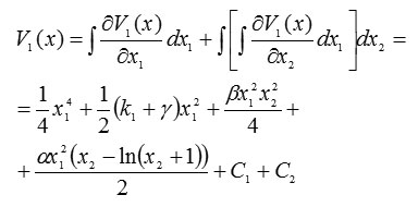
and

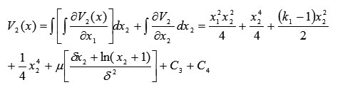
Thus, the Lyapunov function takes this scalar form:

However, the Lyapunov function V(x) is not positive definite because it contains negative components (terms of odd degree). Hence, we need to find the conditions under which the Lyapunov function is positive definite.

To do so, we next build the Hessian matrix of the Lyapunov function:

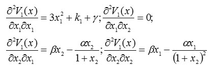
and

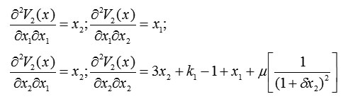
Thus, the Hessian matrix is

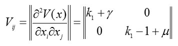
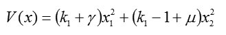
At point (0;0), the Lyapunov function in square form is

and the conditions for being positive definite are given by

At another stationary point (M;0), the matrix Hessian is

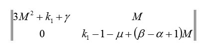
and at this point, the Lyapunov function is

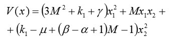
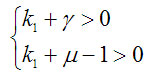
Then the conditions for positive definiteness of the square form are

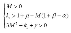
From the condition  and the definition of M below (2), the parameters satisfy  and . They are also real.

Thus, we have found conditions for the parameters under which our Lyapunov function is positive definite and its time derivative is negative definite. These conditions identify an area of robust stability for dynamical system (2) [14]. This means that system (2) captures system states in which tumors do not continue to grow.

Boomerang Effect

Although the model in (2) includes situations in which tumors do not grow, in clinical practice, we know that many tumors initially respond well to treatment, but after a short time, they start to grow again. That is, once a chemical treatment has started, some tumors may adapt; hence, the treatment is no longer effective. We call this the “boomerang effect” [7]. Clinically, protective measures must be repeated regularly to avoid the boomerang effect. If protective measures are not regular, there will be time for tumor cells to adapt to chemical treatments.

To exclude the “boomerang effect” in our mathematical model, we consider the following model:

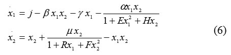
where the fractional terms describe loss changes. Now we add D-faсtor terms to system (6):

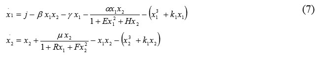
Thus, with the D-factors, we exclude the boomerang effect and can control the growth of cell numbers resulting from uncontrolled cell proliferation. Phase portraits for system (7) appear in Fig. 7.

Results and Discussion 

In this section, we illustrate the behavior of each of the above models for selected values of their parameters. Figure 5 shows results from system (1) when its six parameters have these values:

The stationary point at x₂ = 0, x₁ ≠ 0 represents zero concentration of cancer cells, that is, complete recovery of the organism.

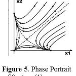Figure 5: Phase Portrait of System (1).   Click here to View figure

 

Figure 6 shows calculated results for system (2) using parameter values

The values for the first six parameters are the same as those used for system (1) above; the difference is only in the seventh parameter. Figure 6 also shows a stationary state that represents a complete cure (x₂ = 0).

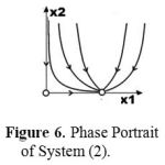Figure 6: Phase Portrait of System (2).   Click here to View figure

 

Results for system (6) are also shown in Fig. 5 for the following parameter values:

Figure 7 contains results for system (7). Figure 7a pertains to these parameter values:

In Fig. 7b, the results are for the same parameter values, except that the value of parameter J was increased from 10 to 20.

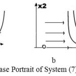Figure 7: Phase Portrait of System (7).   Click here to View figure

 

In both Figs. 7a and 7b, a complete cure is possible, but in Fig. 7b, the cure requires a higher concentration of effector cells (response of the immune system).

Conclusions

This paper has reported on mathematical methods for modeling and controlling growth of tumor cells in living cancerous tissues. The models are pairs of nonlinear differential equations that include terms to account for growth of tumor and effector cells, control of cancerous growth by effector cells, natural mortality of both kinds of cells, and suppression of the boomerang effect in cancer treatments. Control of tumor growth and exclusion of the boomerang effect were modeled using one-parameter mappings (D-factors).

In general, phase portraits from the models exhibit one or two stationary states (see Fig. 2). The first represents cancer treatment that reduces the concentration of tumor cells to zero: complete recovery of the organism. The second stationary state is a “frozen” state that represents treatment in which the tumor is not eliminated, but its growth can be controlled at the expense of effector cells (the immune system).

In the case of model system (2), we could construct the Lyapunov function and identify the region of stability in terms of model parameters. In physical terms, this means that the parameter controlling tumor growth somewhat decreases the population of effector cells. In biological terms, it means that for the system to be stable, the growth of effector cells () must be positive, i.e., there should be enough protein in the cells. Furthermore, interactions between parameters that represent natural mortality rates of the tumor and effective cells (and) are essential. Therefore, effector cells have to be chemo-stable.

We also demonstrated that by introducing a D-factor into models, we can exclude the boomerang effect. The boomerang effect occurs in some cancer treatments in which tumor growth is initially reduced, but the tumor adapts to the treatment, and the tumor resumes growth.

More generally, this paper illustrates that the “compensatory effect” can be applied to control the growth of tumor cells in an organism [15, 16], fixing the immune system at a predictable level [17, 18]. Furthermore, with the help of regulating factors, it is possible to evaluate the level to which populations of tumor cells can be controlled [19, 20].

These results should motivate new theoretical studies on the medical-biological treatment of tumor cells and on the regulation of the immune system. These studies are especially important for the prevention and early intervention of cancer.

Acknowledgments

Special thanks Professor Khlebopros R.G., Professor Beisenbi M.A, As. Prof. Nikulin V.V., As. Prof, Ph.D. Omarov A.N. for fruitful discussions on the biological and mathematical implications and possible extensions of the work.

References

1. Adimya, M. and Crauste, F. Mathematical model of hematopoiesis dynamics with growth factor-dependent apoptosis and proliferation regulations. Comput. Model. 49 (2009) 2128-2137.
2. Roeder, I., Herberg, M. and Horn, M. An “age”-structured model of hematopoietic stem cell organization with application to chronic myeloid leukemia. B. Math. Biol. 71(3) (2009) 602-626.
3. Kim, P.S., Lee, P.P. and Levy, D. Modeling imatinib-treated chronic myelogenous leukemia: reducing the complexity of agent-based models. B. Math. Biol. 70(3) (2008) 728-744
4. Kim, P., Lee, P. and Levy, D. A PDE model for imatinib-treated chronic myelogenous leukemia. B. Math. Biol. 70 (7) (2008) 1994-2016.
5. Roeder, I., Herberg, M. and Horn, M. Modelling repeated epidemics with general infection kernels. Res. Lett. Inf. Math. Sci. 6 (2004) 159-170.
6. Bazykyn, A.D. Nonlinear Dynamics of Interaction of Population, Moscow 2003.
7. Khlebopros, R.G., Isaev, A.S. and Nedorezov, L.V. Dynamics of wood insects number. Novosibirsk. Sciene, 1984.
8. Khlebopros, R.G., Okhonin, V.A. and Fet, A.I. Catastrophes in Nature and Society, Volume 1, 2010.
9. Nikolis, G. and Prigogine, I. Exploring complexity: an introduction, Moscow, 1990.
10. Poston, T. and Stewart, I. Catastrophe Theory and its Applications, Dover Publications, 1996.
11. Boris, T.P. Introduction to optimization. Optimization Software, Inc. Publications Division, New York, 2010.
12. Liapunov Functions and Stability in Control Theory. Bacciotti, Andrea, Rosier, Lionel. Originally published as volume 267 in the series “Lecture Notes Control” by Springer, London, 2001, 2nd ed., 2005, XIV, 238 p. 20 illus.
13. Schwartz, L. Analyse Mathematique. Hermann, Vol. 1. Part IV. №8, 1967.
14. Beisenbi, M. A., Kulniyazova, K. S. Determining the region of robust stability of control systems via Lyapunov functions, in: The Proceedings of the VIth International Asian School-Seminar. Siberian Branch Russian Academic Science Novosibirsk, 2010.
15. Yermekbayeva,    J.J. and Omarov, A.N. Compensatory effect for controlling the population of phytophages and enthomophages, Eurasian Entomological Journal 9(3) (2010). http://www.euroentjourn.narod.ru/indexrus.html
16. Yermekbayeva, J.J. The doctoral thesis. The analysis and research of complex behaviour population models. ISBN 9965-31-334-4, L.N.Gumilyov Eurasian National University, Reviewer: R.G.Khlebopros (2010).
17. Yermekbayeva, J.J. Use of one-parametrical structural-steady steady mapping for control of system predator-prey. Bulletin of L.N.Gumilyov Eurasian National University, 2010, Vol.4. http://repository.enu.kz/xmlui/bitstream/handle/123456789/83/ispolzovanie_odnoparametricheskih.pdf?sequence=1.
18. Yermekbayeva, J.J. The Influence of structural and steady displays in competition models. The proceedings of the Perspektywiczne opracowania są nauką i technikami – 2011: materiały vii iędzynarodowej naukowi-praktycznej konferencji, Przemyśl, 2011.-V.11. S.15-20. http://www.rusnauka.com/28_PRNT_2011/Economics/8_94027.doc.htm
19. Yermekbayeva, J.J. Control of tumoral cages growth with the help of «compensatory effect». The proceedings of the XVI All-Russia symposium with international participation «Complex systems in extreme conditions», Krasnoyarsk scientific center of the Siberian Branch of the Russian Academy of Science, 2012.
20. Abitova, G., Nikulin, V., Beisenbi, M. and Ainagulova, A. Control System with High Robust Stability Characteristics Based On Catastrophe Function. The proceedings of the ICECCS’ 12. 2012.

(Visited 99 times, 1 visits today)