C. Anjanappa¹ and H. S. Sheshadri²

¹Department of Electronics and Communication Engineering, The National Institute of Engineering, Mysore, Karnataka, India.

²Department of Electronics and Communication Engineering, PES College of Engineering, Mandya, Karnataka, India.

Corresponding Author E-mail: anjanappagayathri@gmail.com

DOI : https://dx.doi.org/10.13005/bpj/1589

Abstract

For proper modelling of signal and noise in MR data requires proper interpretation and analysis of data, the different approaches with this degradation due to random fluctuations in the MR data, probabilistic modeling is power solution, which needs correctness in the computation of noise is challenging task and various stastical approaches can be utilized. After modelling the noise it can be integrated to denoising pipeline, in this research work, the recognition of noise only pixels and the evaluation of standard deviation of noise using median, mean or other optimal sample quantiles are combined in to single frame work for noise assement and uses fixed point iterative procedure to obtain standard deviation of noise. We tested the effectiveness of the algorithm to the MR clinical and synthetic data base.

Keywords

Gamma Distribution; Noise Estimation; Parallel Reconstruction Algorithm; Rayleigh Distribution

Download this article as: 

Copy the following to cite this article: Anjanappa C, Sheshadri H. S. Probabilistic Identification and Estimation of Noise: Application to MR Images. Biomed Pharmacol J 2018;11(4).

Copy the following to cite this URL: Anjanappa C, Sheshadri H. S. Probabilistic Identification and Estimation of Noise: Application to MR Images. Biomed Pharmacol J 2018;11(4). Available from: http://biomedpharmajournal.org/?p=24105

Introduction

Noise assement in MRI ^1,2,3 usually requires the assessment of standard deviation of noise. Earlier methods can be separated into two methods for the computation of noise, first method involves the manually selected region of interest (ROI), in the second method entire volumetric data or image is considered for estimation without human interpretation. The problem is facing for the current automatic estimation method is separation of original signal from noise effected signals and other in homogeneity artifacts^4,5 the proposed work of two authors is by aggregate the values of all pixels from an entire pixel data set in to one dimensional array and estimate the standard deviation of noise from the histogram of one dimensional array.in this research work, introduce simpler method for noise assement in MR image to eliminate the drawback of two authors. The proposed method requires the recognition of noise only pixels which enhance the performance and accuracy of estimation of Gaussian noise and requires the prior knowledge about the standard deviation of Gaussian noise, and can cater distribution of noise for further analysis like segmentation and registration. Most of the noise estimation algorithms in the earlier method is based on background methods and object based methods, background methods which follow Rayleigh distributed noise and object based methods follow Gaussian and rician noise.⁶ In this work we developed an algorithm for noise assement in MRI for the data acquired for multiple N receiver coils in which data follows nc- distribution is the special case of Rician distribution.⁷ Recently the author Rajan^7,11 developed an algorithm for the estimation of noise without background. Most of the above estimation algorithms are developed are sensitive to artifacts results in inaccuracy of noise estimation, the author coupe⁸ developed robust noise estimation algorithm rician median absolute deviation [RMAD] for noise bias correction and artifacts to achieve accurate noise estimation, Other methods of noise estimation is variance stabilization transformation framework (VST) for bias inhomogeneity^12,13 correction in  MR image to transform bias Rician noise distribution in to uniform Gaussian distribution and achieves accuracy noise estimation compared to other noise estimation methods.

Materials and Method

The data set obtained from the DIPY (diffusion imaging in python) and JSS hospital Mysore Karnataka, India.

Data set 1

STANFORD_HARDI (High resolution Diffusion Weighted imaging dataset (N=4)) Uses phased array coil system and SOS reconstruction (without parallel imaging).

TAIWAN_NTU_DSI (Diffusion Spectrum imaging) Dataset (N=1) uses phased array coil system and SENSE reconstruction. (With parallel imaging).

Dataset 2

Philips 3.0 Tscanner

MRI T1 weighted axial Brain image having pathology acquisition parameters are TR=5.3sec, TE=20ms, slice thickness=3.5mm, Resolution of 512×512. Parallel Image Reconstruction: SENSE.

Philips 3.0Tscanner

MRI T1 weighted sagittal Brain image with acquisition parameters are TR=5.3 sec, TE=20ms, slice thickness=3.5mm, Resolution of 512×512. Parallel Image Reconstruction: SENSE.

Diffusion Imaging in Python (Dipy) is a free and open source software project tool where image processing library tools are available for the analysis of data from diffusion magnetic resonance imaging (dMRI) experiments.

Method

Noise modelling in MRI

The MR data acquired from the multiple N receiver coils m (or m_{i j k}) follows non-central chi distribution [10] which is reconstructed from sum-of-squares algorithm (SOS) distribution,

distribution of 2N degrees of freedom with the non- centrality distribution parameter is given by

η² /σ_g². The probability density function (PDF) of

is given by [9]

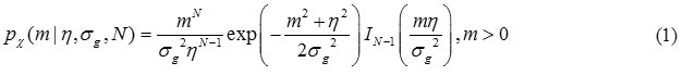
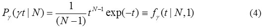
Where the PDF is zero for m < 0, η is the underlying (combined) signal intensity, σ_g is the standard deviation of Gaussian noise and I_k is the kth-order modified Bessel function of the first kind. We should note that magnitude MR signals reconstructed from other parallel image reconstruction techniques may not follow non-Central Chi distribution, Note that when N= 1, Eq. (1) reduces to the Rician PDF [2].

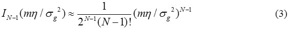
In this research work, the PDF of magnitude noise (i.e. η =0) is more relevant than the PDF of magnitude signal (η ≠ 0). Therefore, we will derive the PDF of magnitude noise from Eq. (1) by setting the input signal to zero, i.e. η =0, then it shows that  PDF of magnitude noise is given by

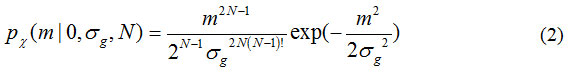
After I_N-1 in Eq. (1) is replaced by first term Taylor expansion about input signal η =0,

Expressed by the following expression

When N=1, Eq. (2) simplifies to Rayleigh PDF.

Then by a change of variables from m to

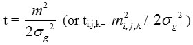
shows that variable t follows form of the particular Gamma PDF

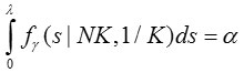
The Gamma PDF, f_y as defined in [31]:

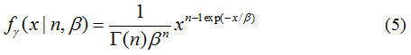
and Γ is the Gamma function.

Distribution of the Mean of Several Sampling Observed M-Values

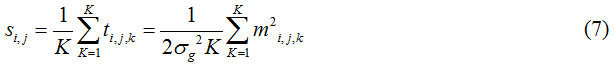
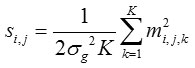
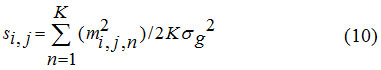
The measurements m _{i, j, k}’s are defined in Eq. (2). We have chosen the arithmetic mean for the identification of noise-only pixels. If knows the distribution for the mean, which is depends on σ_g, we can decide for any observed mean sample came from the noise-only distribution. Which will provide the expression for the arithmetic mean of the several sampling observed values of m _{i, j, k} s through the method of Characteristic function. In short, the derived random variable s_{i, j} representing the arithmetic mean of K independent Gamma Random variables {t_i,j,1, t_i,j,2,…. t_i,j,k} is given by

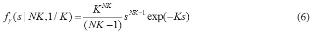
Further, the new random variable s_{i ,j} related to K independent magnitude MR measurements, {m_i,j,1, m_i,j,2, m_i,j,k} drawn from  the distribution of magnitude noise is given by

Identification of the noise-only pixels using probabilistic method requires to define threshold on ‘s’  i,e upper and lower threshold, so that a given proportion of all noise-only voxels or pixels fall between these two values. And we need to derive the cumulative distribution function (CDF), and it’s inverse of the distribution of  ‘s’ to specify the lower and upper threshold values of s. Assume that N and K are known and the initial estimate of σ_g, is required, is obtained by automatically using the simple search method are below.

The probability distribution function and CDF of  ‘s’ is denoted by

the inverse of CDF ‘s’ are denoted symbolically by λ= p_s ^-1 (a | N, K).

The CDF of ‘s’ and its inverse are given by

λ= p_s ^-1 (p_s ( λ| N, K).| N, K) and a = p_s^-1 (p_s ( a| N, K)| N, K) Note that  P_s^-1 (a|N,K) given by Inverse Gamma Regularized [NK,1-α]|K  in Mathematica[14].The lower and upper threshold values of ‘s’ are λ _–, λ ₊ denoted  probabilities are a/2 and 1-(a/2) can be expressed in terms of the inverse CDF of ‘s’ given by λ _– = P_s^-1 (a/2|N,K), and  λ ₊ P_s^-1 (1-a/2|N,K), Thus, a collection of K independent magnitude MR signals {m _i,j,1, m _i,j,2, m _i,j,k}  from the acquisition  is decided to contain only noise if

which  satisfies the inequalities, λ _– ≤ S _i,j, ≤ λ ₊.

Noise Estimation using the sample median, the sample mean or optimal quantiles method

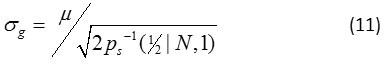
The computation of Gaussian noise SD is obtained from the simple method of mean, denoted by <m>, of means of a collection of acquisition data measurements. The estimation of Gaussian noise SD, σ_g, can also be computed from the sample quantile of a unique optimal order α*

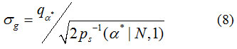
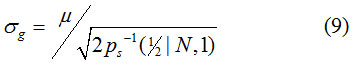
Note that both the sample median and the median of the continuous PDF, Eq. (2), are denoted by the same symbol. Note also that the denominator of Eq. (9) can be computed in advance, see Table 2. For example, when N = 1, Eq. (9) can be expressed mathematically

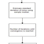Figure 1: Block diagram of PIESNO Algorithm.   Click here to view figure

 

Algorithm Implementation

Input parameters:    N, K, λ _–, λ₊, m _i,j,k  for all input measurements, the estimate of σ_g, is needed

Output framework:  identification of noisy only pixels and estimate of σ_g, and array of noise elements ‘Ω’

Step 1 is the identification of noise-only pixels, and dynamically adding noisy pixels in to new elements of the one-dimensional array, Ω. And compute the standard deviation of noise in advance using the equation shown below.

At each pixel location (i,j), compute s_i,j:

A positive identification is made if S _i,j satisfies the condition  λ _– ≤ S _i,j, ≤ λ ₊.

In Step 2, the channel between the identification and estimation of noise-only pixels is set and create one-dimensional array of Ω, which is the union of all the arrays of K measurements identified as noise only pixels. Note that the number of positive identifications is defined is equal to the number of the positively identified arrays. Finally, the sample median of Ω, 1, is selected. Note again that the sample mean of Ω or the sample quantile of Ω of a specific order may be used here.

Step 3 is the computation of standard deviation of noise, the array of sample median, l, of  Ω computed in Step 2 is used to estimate σ_g. Note again that the sample mean and other optimal quantiles are defined below.

In Step 4, if the iteration stops the Ω is empty, which repeats procedure from Steps 1 to 4 sequentially until convergence or the maximum number of iterations is reached. Here, a sequence of estimates of σ_g produced by the iterative procedure is considered if the absolute difference between any successive estimates is less than small number, say 0.00000000001.

Step 5, the noise identification and computation of the standard deviation of noise  is denoised using NLM algorithm and evaluate its performance parameters.

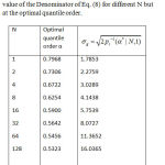Table 1: The optimal quantile value for different N and the value of the Denominator of Eq. (8) for different N but at the optimal quantile order.   Click here to view table

 

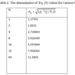Table 2: The denominator of Eq. (9) values for various N.   Click here to view table

 

Results and Discussion

The proposed algorithm is implemented using Python. After the python implementation of the PIE S. NO we plot the SD of noise-only pixels using MATPLOTLIB with N (phased array coils) varying from 1 to 12. The figure (4-6) below shows the plots of PDF of noise-only pixels vs SD (sigma) with N=1, 4 and 10. Using different data sets below.

Piesno Results for Different Datasets

Tested on Taiwan and Stand ford Dataset

Fig.2 and fig.3 shows the data set obtained from Stanford_hardi dataset acquired using 4 phased array coils. In these images the White dots appearing in the image are the noise-only pixels identified and estimated using our proposed PIESNO algorithm. These noisy only pixels are denoised using well known NLM algorithm using python. The image is subjected to denoising with Background preservation. Similarly the data set obtained from Taiwan dataset acquired using single phase array coil, from these two graphs we observed that the noise identified is Rician and Gaussian from the background region and it is well modelled by Gaussian and rician from the PDF curve is as shown in fig.4 and fig.5.

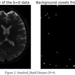Figure 2: Stanford_Hardi Dataset (N=4).   Click here to view figure

 

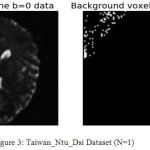Figure 3: Taiwan_Ntu_Dsi Dataset (N=1).   Click here to view figure

 

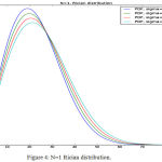Figure 4: N=1 Rician distribution.   Click here to view figure

 

From the algorithm the estimated value of standard deviation of noise and its PDF curve is shown in fig.4 above. The curve is not symmetric about a mean value. Hence we identify the noise present in the MRI as Rician Noise or nc-λ distribution.

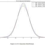Figure 5: N=4 Gaussian distribution.   Click here to view figure

 

For the fig.4 above estimated value of standard deviation of noise using PIESNO algorithm using N=4, the plot obtained is a symmetric curve as shown above. The curve is symmetric about the value 0. Hence it follows a normal distribution and the noise is identified as a Gaussian Noise.

Similarly for N>1, the plot follows the same curve as shown below fig.5 for N=10.

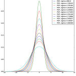Figure 6: N=10 Gaussian distribution.   Click here to view figure

 

Thus we can interpret the results of PIESNO as

For N=1 the noise estimated and identified is Rician Noise.

For N>1 the noise estimated and identified is Gaussian Noise.

Tested on Clinical Data

Fig.7  shows the data acquired from MR machine (clinical data) using multiple phase array coils using parallel image reconstruction SENSE algorithm and fig. 8  shows data acquired using SOS reconstruction algorithm without subsampling. The identification of noise distribution using PIESONO algorithm and its results with histograms is as shown in fig. 9-12, from this graphical analysis found that the noise distribution is Gaussian and rician.

The denoising results of the algorithm for Taiwan and stand ford dataset are shown in fig.13 and fig.14 and difference image (Residual image) is shown, it is observed that the algorithm shows better preservation of edge and efficient noise reduction.

The comparison of denoising algorithm with other algorithm is shown in table 3. From this table it is observed that the NLM algorithm shows efficient noise reduction with others and it is verified from PSNR values, and it is burden due to long execution time compared with AONLM and PCA algorithm is shown in the table 3.

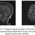Figure 7: MRI T1 Weighted sequence images in the axial and sagittal view acquired using multiple Phase Array coils (parallel image reconstruction: SENSE).   Click here to view figure

 

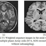Figure 8: MRI T1 Weighted sequence images in the axial view acquired using multiple phase Array coils (N=4, SOS reconstruction without subsampling).   Click here to view figure

 

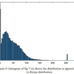Figure 9: Histogram of fig.7 (a) shows the distribution is approximated to Rician distribution.   Click here to view figure

 

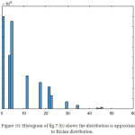Figure 10: Histogram of fig.7 (b) shows the distribution is approximated to Rician distribution.   Click here to view figure

 

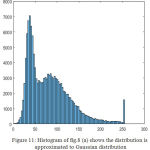Figure 11: Histogram of fig.8 (a) shows the distribution is approximated to Gaussian distribution.   Click here to view figure

 

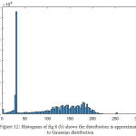Figure 12: Histogram of fig. 8 (b) shows the distribution is approximated to Gaussian distribution.   Click here to view figure

 

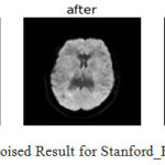Figure 13: Denoised Result for Stanford_Hardi (N=4).   Click here to view figure

 

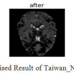Figure 14: Denoised Result of Taiwan_Ntu_Dsi (N=4).   Click here to view figure

 

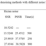Table 3: The comparison of denoising methods with different noise levels on MR T1 weighted Images.   Click here to view table

 

Discussion

Earlier estimation algorithms work for single image but our proposed algorithm is well suited for multiple images to estimate the variance of noise and it is not suited for clinical practice requires longer acquisition time to estimate the level of noise. Our method is applicable to larger class of magnitude data measurements acquired from the MR machine than Rayleigh-distributed data (i.e., N = 1) and discuss some limitations of the proposed approach. PIESNO cannot be expected to perform well for very small K because the identification of noise may be less stable and may not produce sufficient number of elements for the estimation of noise via the median method to be useful as an estimator. We tested the effectiveness of the algorithm with clinical and synthetic database and conclude that stastical distribution of noise is Gaussian, rician or nc-λ distribution and it is verified from mathematical derived probabilistic distribution function. The denoising performance of the algorithm is compared with standard conventional algorithm and execution time.

References

1. Macovski. Noise in MRI, Magn. Reson. Med. 1996;36:494–497.
   CrossRef
2. Gudbjartsson H.,Patz S. The Rician distribution of noisy MRI data.Magnetic Resonance in Medicine. 1995;34(6)910–914.
   CrossRef
3. Drumheller. General expressions for Rician density and distribution functions. IEEE Trans. on Aerospace and Electronic Systems. 1993;29(2):580–588.
   CrossRef
4. Sijbers.,  den Dekker J. A., Van Verhoye A. M.,Van Dyck D. Estimation of the noise in magnitude MR images. Magn. Reson.Imag. 1998;16(1):87–90.
5. Sijbers., Poot D., den Dekker A. J and Pintjens W.  Automatic estimation of the noise variance from the histogram of a magnetic resonance image. Physics in Medicine and Biology. 2007;52(5):1335-1348.
   CrossRef
6. Aja-Fernandez., Niethammer M., Kubicki M., Shenton M. E and Westin C. F. Restoration of dwi data using a rician lmmse estimator. Medical Imaging. IEEE Transactions on. 2008;27(10):1389-1403.
7. Aja-Fernandez.,  Alberola-Lopez C and Westin C. F. Noise and signal estimation in magnitude MRI and Rician distributed images: a LMMSE approach. IEEE transactions on image processing.  2008;17(8):1383-1398.
   CrossRef
8. Sijbers.,  den Dekker A.,  Scheunders P.,Van Dyck D. Maximum-likelihood estimation of Rician distribution parameters. IEEE Trans. Med.Imaging. 1998;17(3):357–361.
   CrossRef
9.  Koay G., Basser P. J. Analytically exact correction scheme for signal extraction from noisy magnitude MR signals.Journal of Magnetic Resonance. 2006;179(2):317–322.
   CrossRef
10. Aja-Fernandez., Tristan-Vega A.,  Alberola-Lopez C. Noise estimation in single- and multiple-coil magnetic resonance data based on ´statistical models. Magn. Reson. Imag. 200;27:1397–1409.
11. Rajan.,  Poot D., Juntu J.,  Sijbers J. Noise measurement from magnitude MRI using local estimates of variance and skewness. Physics in Medicine and Biology. 2010;55(16):441.
    CrossRef
12. Coupé P.,  Manjón J., Gedamu E.,  Arnold D., Robles M and Collins D. L. Robust Rician noise estimation for MR images. Medical Image Analysis. 2010;14(4):483–493.
    CrossRef
13. Foi A. Noise estimation and removal in MR imaging: the variance-stabilization approach,” in [Proceedings of the IEEE International Symposium on Biomedical Imaging: From Nano to Macro]. 2011.
    CrossRef
14.  Wolfram S. The Mathematica Book, Wolfram Media, Champaign. 2003.

(Visited 481 times, 1 visits today)