Hamed Azad, Gholam Abbas Akbarand Gholam Ali Akbari

Department of Agronomy and Plant Breeding Science, College of Aburaihan, University of Tehran, Tehran-Pakdasht, Iran.

Corresponding Author E-mail: azadi.hamed@ut.ac.ir

DOI : https://dx.doi.org/10.13005/bpj/1564

Abstract

Simulation models of crops are used for experimental and complementary research on field projects. These models are also useful for interpreting the results and examining agricultural systems under different environmental and management conditions. The aim of this study was to describe a model for wheat (SSM), guarantee wheat cultivars in a genetic discussion in the Pakdasht environment, and present the results of its evaluation. The model of phenological stages, growth, and aging of leaf area and the production and distribution of dry matter simulates water function and balance. The SSM model simulates the growth stages of the plant in response to environmental factors, heat, and the ability to access solar radiation. In order to evaluate the SSM model, field experiment data of two wheat cultivars—SW and Pishtaz—were used as factorial, based on a randomized complete block design with four replications. Subsequently, the parameters were evaluated, the model was tested in accordance with independent data, and the results indicate its acceptance for the main aspects of crops compared to the observed experiments—for example, for SW, we have 1830 GDD to 2310 GDD from pollination to treatment and extinction factor in Pishtaz is 0.71 and PLAPOW coefficient is 1.6484±.063, which can finally be used to simulate these figures.

Keywords

Crop Model; Simulation; Wheat SSM Model

Download this article as: 

Copy the following to cite this article: Azad H, Akbar G. A, Akbari G. A. Parameterization of SSM Model to Analyze Wheat Growth and Yield Potential Under Pakdasht Conditions. Biomed Pharmacol J 2018;11(4).

Copy the following to cite this URL: Azad H, Akbar G. A, Akbari G. A. Parameterization of SSM Model to Analyze Wheat Growth and Yield Potential Under Pakdasht Conditions. Biomed Pharmacol J 2018;11(4). Available from: http://biomedpharmajournal.org/?p=24373

Introduction

The models of the crops have long been used in many countries to simulate the growth of crops.^1,2 because of the fact that the modeling process of crops is a process that requires a lot of time to estimate the parameters and finally run and evaluate the model. Choosing a better model with more reliable results among the various models of growth and development of crops will save a lot of workload in terms of studies.

It is necessary to analyze the factors that limit genetic factors, including genetic, climatic, soil, water, and potential yield of the plant, to study and investigate ways of increasing wheat yield.³ Such a study and analysis can be carried out using laboratory and field experiments around the world in a few years. As is known, these experiment fields are time-consuming and costly. Today’s information technology makes possible to simulate the climatic, biological, and physical phenomena at different stages of the research; these simulation models allow the application of various scientific aspects, including soil chemistry, soil physics, meteorology, crop physiology, and crop improvement by mathematical equations to predict growth and yield.^4,5 These models are good tools for simulations of crops.^6,7

One important point to consider is that these models are complementary to field experiments and are by no means an alternative to field experiments.⁸ A basic model for wheat can simulate the phenology, dry matter to various plant components and yield. The SSM Model  is used for wheat.⁹ With the help of this model, it is possible to analyze the crops and genetic, environmental, and management constraints.¹⁰

The purpose of this study is to evaluate the efficiency and use of SSM model under Pakdasht conditions and determine the genetic coefficients (parameterization) in SW and Pishtaz wheat cultivars.

Materials and Methods

To simulate the development of wheat yield using the SSM model in the province of Tehran, field experiment data were used in 2016–17 (research farm of Tehran University–Abureihan Campus). In this research, two Pishtaz and SW cultivars were used (as used in Tehran province). Before the experiment, depths of 0 to 30 cm were sampled and the chemical and physical properties of soil were determined. Initially, a germination test was performed for the two cultivars and, after a week, SW had 94% and Pishtaz had 85% vigor. According to the densities considered, 50, 100, 150, 200, and 400 plants per square meter of seeds were accurately counted and spaced 20 cm on the cultivation row.

In this research, traits such as the number of leaves, leaf area, number of green leaves left and fall in the main stem, received radiation ratio, phonological stages, dry weight (green and yellow leaf, stem, pod and seed), plant height, yield, and yield components were measured and calculated.

Phenology

All the stages in the development period were carried out using 10 plants and in accordance with the method of.¹¹ In order to measure dry weight in each sampling (every 10 days), after measuring the leaf area and counting the number of nodes in the main stem, green and yellow leaves, stems, seeds, and shells of pods were separately put in an oven at 70°C to reach constant weight. In order to estimate the radiation received, the radiation meter should be adjusted in accordance with the environment and then the radiation was measured and used in accordance with the method of.¹² An area of ​​around 2 square meters of each plot was harvested once at full treatment stage, where 95% of the wheat was yellow and brown and the seed moisture content was 20%, to determine the yield and yield components.

Now the model is named Triticum model was developed by.¹³ This model has the ability to simulate the phonological stages, leaf growth and decay, distribution of dry matter, formation of yield, and the balance of soil water. The model also simulates the plant’s response to environmental factors like phenoperiod, heat, nitrogen, and radiation on a daily basis and uses the available water-soil-air information.¹⁴  This model does not take into account the effects of diseases, pests, and weeds on the plant. Nevertheless, these factors are not relevant to physiological properties and plant traits.

The quantitative method of predicting phonological growth in wheat was examined as a function of phonological period and temperature in this model.

BD = f(T) × f(P)                        (1)

P= photoperiod function. T= Relative Development Speed

The key phonological stages required to simulate the physiological processes of growth and yield in wheat are as follows (14) :

Planting until germination

Germination to tillering

Stem to seed

Seed to spike

Spike to pollination

Pollination to physiological treatment

Physiological treatment until the harvest

The cumulative thermal time required for one stage is expressed in terms of the minimum number of calendar days required for a physiological stage (BD), which is called the required biological day – a number between zero and one which defines a required day for development.

The relationship: 1 BD = f (T) × f (P)

In this equation, f (T) and f (P) are temperature and phonological period functions respectively, which show the relative velocity of growth in each temperature and phonological period relative to the optimal state.

The relative velocity response of wheat growth to the average daily temperature uses a” tooth-like function”

F(T)     =  (TMP – TBD) / (TP1D – TBD) if                  TBD ˂ TMP ˂ TP1D

(2)       =    (TCD – TMP) / (TCD – TP2D)              if                 TP2D ˂ TMP ˂ TCD

=     1                                                      if               TP1D  TMP  TP2D

=   0                                                        if       TMP  TBD or TMP  TCD

In this equation, TMP is the average daily temperature, Tmax is the maximum daily temperature, Tmin is the minimum daily temperature, F(T) is the temperature Function, TBD is the base temperature, TP1D is the final desired temperature, TP2D is the upper optimal temperature, and TCD is the ceiling temperature. In this survey, the minimum and maximum daily temperature, rainfall, and sunny hours were obtained from measured values from the meteorological station of Mehrabad Tehran including semi dried weather, 20 km from the research field.

The model uses a piecewise function to quantify the reaction of the development rate to the phonological period.

F(P) = 1- PP sen (PP- CPP) if   PP ˃ CPP =    F (p) =  1 PP ≤CPP                       (3)

Where PP is the phonological period (based on hours per day), CPP is the critical phonological period( i.e.), the phonological period which begins to be reduced because of coincidence with short days of the growth, and PP sen is called the phonological period sensitivity factor.

The leaf area

The Figure 1 shows the rate of the appearance of philocrone.¹⁵ The numerical value of the physiological day till the end of leaf growth in the model is considered the end time of leaf growth.

INODE= TU/ PHYL               (4)

In this equation, TU is daily thermal temperature and PHYL is degree days. To calculate the total number of nodes per plant (MSNN), the increased number of nodes per day (INODE) is used in the model. For this, the number of nodes per day is summed up with the number of nodes on the previous day (MSNNi-1). Therefore, the total number of nodes per plant before TLM is equivalent to MSNNI.

MSNNi= MSNN_i-1+INODE             (5)

The leaf area is P(A) per square meters in the plant by MSNNi. In this way, allosteric regulation between the number of leaves per plant and leaf area is used, which is a power (13).

PLA = PLACON × MSNN ^PLAPOW               (6)

In this equation, PLAPOW and PLACON are constant coefficients. In the daily increase model, the leaf area index (GLA) is calculated by increasing the plant leaf area and density (PDEN):

GLAI = (PLA_i — PLA_i-1) × PDEN / 10000                       (7)

In this equation, PLAi is the current day leaf area and PLAi-1 is the cumulative leaf area of the day before. The coefficient of 10,000 has been added to convert GLAI from centimeters per square meter per day to square meters per square meter per day.

The daily reduction in leaf area index in the model is calculated as follows:

DLAI = DTT / (ttMAT – ttBSG) × BSGLAI                  (8)

DLAI= leaf area index scale. MAT= total thermal time from planting until harvest.

BSG= from planting until beginning of grain growth stage.BSGLAI=leaf area index in beginning of grain growth stage.

The leaf area index

Finally, leaf area index by increasing GLAI and Daily DLAI in the model can be calculated as follows:

LAl_t = LAI_t-1 + GLAI – DLAI                 (9)

Dry Matter Production

In this model, dry matter production is predicted by a simple RUE-based method.(Photosynthetic Active Radation) PAR value received per day is obtained from the leaf area index and KPAR. KPAR value was considered constant for the entire growth season. The amount of dry matter produced per day is obtained from PAR multiplication received by RUE. RUE is moderated for the average daily temperature and CO₂ concentration.¹⁶

To calculate the dry matter production per day, calculating the fraction of PAR input received by the crop canopy (FINT) is necessary. This fraction is simply calculated by using an exponential equation between radiation and receipt, which is calculated in accordance with Beyer-Buger-Lambert rule¹⁷:

FINT = 1 – exp (– KPAR × LAI)                   (10)

In this equation, KPAR is the light extinction factor.

Though RUE is a constant under favorable growth conditions, inappropriate temperatures can reduce it.¹⁸ For this reason, RUE value is adjusted to the basic daily temperature. RUE correction factor for temperature (TCFRUE) in the model is calculated using the following equation:

TCFRUE = 0 if TMP ≤ TBRUE

(TMP-TBRUE) / TPIRUE – (TBRUE if  TBRUE <TMP<TPIRUE

TCFRUE =1 if TP2RUE ≤ TMP ≤ TP1RUE

TCFRUE = (TCRUE -TMP) / (TCRUE- TP2RUE) if TP2RUE<TMP<TCRUE                      (11)

TCFRUE like f(T) changes from zero to 1, and, in fact, this factor shows RUE value at any temperature relative to the optimal temperature. TP2RUE, TPl RUE TBRUE, and TCRUE are cardinal temperatures for RUE and respectively show the base temperature, lower desired temperature, upper desired temperature, and ceiling temperature. Thus, the model calculates RUE value for each day of RUE under desired conditions (IRUE) and TCFRUE:

RUE = IRUE × TCFRUE                           (12)

The model is calculated with received PAR fraction and RUE of daily dry matter production (DDMP) as follows:

DDMP = PAR × FINT × RUE                   (13)

Finally, the total dry matter produced (WTOPi) is calculated by adding the dry matter produced per day to the accumulated dry matter (WTOPi-1) as follows:

WTOP_i = WTOP_i-1 + DDMP            (14)

Dry Matter Distribution

In the SSM model, a simple method is used for distributing dry matter. In this method, first, the reservoirs for the dry matter and the developmental stages in which the reservoirs are active should be identified. Three reservoirs are considered:

(1) leaves, (2) stems, and (3) seeds

From the stage of emergence to the beginning seed growth (BSG), the daily dry weight gain of leaves (GLF in grams per square meter per day) is affected by the daily production of dry matter (DDMP in grams per gram / m² / day) and allocation factor to the leaf (FLF in grams per gram). The amount of daily dry production that is not present on the leaves will be allocated to “stems” (GST; stem growth rate in grams per square meter per day):

GLF = DDMP × FLF              (15)

GST = DDMP – GLF                (16)

The dry matter allocation factor to the leaf in the developmental period from the end of the leaf growth to the beginning seed growth (FLF2) can be estimated as follows:

(FLF2) = (BSGLDM – TLGLDM) / (BSGDM – TLGDM)            (17)

In this equation, BSGLDM and TLGLDM are the leaf dry weight and BSGDM and TLGDM are the dry weight of the whole wheat plant at two stages of BSG and TLM.

Formation of yield

The modeling of the seed growth rate and the formation of yield on the basis of the concept of linear increase in the harvest index^9,19 is modified by.²⁰ The seed growth rate per day (SGR) (g / m² / day) is calculated as follows (13):

SGR = DHI × (WTOP_i-1 + DDMP_i) + DDMP_i×HI_i-1                       (18)

Here, HI is the harvest index, DHI is the increase in daily harvest index in the linear phase of the seed growth, WTOP is the total dry weight (g / m²), and DDMP is the daily dry matter production rate. In the model, the first daily total dry matter produced (DBP) is added to the dry weight of the vegetative components, and then the seed growth rate is deducted from the dry weight of the vegetative components, i.e.:

WGRN_i = WGRN_i-1+SGR                                              (19)

WVEGi = WVEG_i-1 + DDMP – (SGR / GCF)              (20)

WTOP_i = WGRN_i + W VEG_i,                                         (21)

where GCF is the seed conversion factor and, in fact, indicates the difference in energy content between vegetative (WVEG) and reproductive tissues (WGRN). The actual value of the gradient of the increase in the harvest index (i.e. DHI) with respect to the maximum value of this gradient (PDHI), the total dry matter at the beginning seed growth (BSGDM) is calculated for the growth season in the simulation. This correction is based on the suggestion of (13). In the model, a tooth-like function was used to calculate the relative gradient of the increase in the harvest index (DHIF). To use this function, the critical quantities of dry matter are required at the beginning seed growth (WDHI). Therefore:

DHIF = 0  if  BSGDM ≤WDHI1

DHIF = (BSGDM – WDHI1) / WDHI2 – WDHI1 if  BSGDM ≤ WDHI1

DHIF = 1 if WDHI2<BSGDM<WDHI3

DHIF = (BSGDM – WDHI) / (WDHI4 – WDHI3) if WDHI3< BSGDM<WDHI4

DHIF = 0 if WDHI1>BSGDM                              (22)

Multiplying DHIF by PDH I yields the DHI value for the growth season while simulating.

In this model, the total dry matter for Total Crop Mass at Beginning Seed Growth (TRLDM) (Translocateable to) and seed growth is obtained from multiplying the fraction of Crop Mass at Beginning Seed Growth by the beginning seed growth (FRTRL) (Translocateable to the grains) in the amount of Crop Mass at Beginning Seed Growth (BSGDM).

TRLDM = BSGDM × FRTRL               (23)

During the seed growth, if the daily amount of dry matter production is less than the seed requirement (i.e. SGR), the shortage is obtained from the difference between the modified seed growth rate for dry matter energy (SGR / GCF) and daily dry matter production (DDMP). This is the same as TRANSL.

FRTRL value is obtained from the test data as follows:

FRTRL = (BSGDM – NGYLD) / BSGDM)                (24)

NGYLID = BYLID – GYLD                                           (25)

In this equation, BSGDM is the total dry weight of the plant in GYLD, BSG is the seed yield, NGYLD is dry weight of organs other than seeds, and BYLID is dry weight in physiological treatment.

Results and Discussion

During the growth period of wheat at the time of performing the test, the average maximum and minimum daily temperatures were 18.6 and 4.9°C respectively. Rainfall during the growing season at the time of performing the test was .96 millimeters . The radiation level at the time of performing the test was not noticeable from November to May.

Estimation of SSM model parameters

Phonological growth

The values ​​of the parameters necessary to quantitate the reaction to temperature using a tooth-like function, such as base temperature, desired lower temperature, desired upper temperature, and ceiling temperature—also known as cardinal temperatures—were considered to be 0, 25, 28, and 40, according to the available references (Table 1) (8).

Table 1: The values ​​of cardinal temperatures, critical day length and phonological period sensitivity coefficients for soybean cultivars (TMP, mean temperature, TBD, base temperature, TPD, desired temperature, TPID, desired lower temperature, TP2D, desired upper temperature, TCD, ceiling temperature; CPP, critical phonological period, and ppsen are phonological sensitivity coefficients).

Parameter	TBD	TPID	TP2D	TCD	CPP	ppsen
Wheat	0	28	25	40	14	17	(soitani and sinclar, 2012)

 

Thermal time for cultivars

Cultivars	Planting until germination	Germination to tillering	Tillering to stem growth	Stem to seed growth	Seed growth to spike	Spike to pollination	Pollination to physiological treatment	Physiological treatment to harvest
SW	267.7	490.41	911.66	1275.8	1438	1595	1830	2310
Pishtaz	276.25	496.41	926.25	1297.7	1509	1646	1830	2310

 

Changes in the leaf area

Estimation of philocrone

To quantify changes in the number of leaves per plant in comparison with the cumulative thermal time (determination of philocrone parameter), in this study, the two-part nonlinear regression model was used (Equation 1). The model contains two cross lines, the slope of the line in the first part indicates an increase in the number of leaves and a horizontal line indicates the maximum number of leaves per plant.

y = a +bx  if x< x^o

y = a +bx_o if x ≥ x                           (1)

where y is the number of leaves in the main stem, x is time (accumulated growth day after planting), a is the curve contact point with a vertical axis (x = 0), b is linear increase rate in the number of leaves (leaf per unit increase in temperature unit), x0 is the time of the linear increase in the number of leaves, and a + bx0 shows the maximum number of leaves in the main stem. Also, with y = 0 in the equation y = a + bx, the degree of growth day after planting, in which the production of leaves starts in the main stem, is calculated as -a / b(18) . The fitting of Eq. (1) was done separately for cultivars and densities.

Table 2: The coefficients a and b and x0 value, the relationships between the number of nodes (or leaves) per plant versus the accumulated temperature unit in the cultivar Sahar, and RMSE DPX root mean square error and R² are the coefficients of determination.

Cultivars	x0 se			RMSE	R2
SW	64.17  1462.2	1.06  -9.4226	0.0014  0.0289	5.69	0.8
Pishtaz	35.78 1496.4	0.6687 -11.66	0.0009 0.0331	3.57	0.93

 

95% of cultivars showed a significant difference found between the coefficients of the equation in different densities and cultivars. Fig. 2-4 shows, for example, the relationship between the number of leaves in the main stem and accumulated thermal time. The end times of linear increases in the number of leaves for Pishtaz and SW cultivars were 1496.4 and 1462.2 time units respectively figure 1. The rate of increase of each leaf per unit of increase in the temperature unit for Pishtaz and SW cultivars was 0.0331 ± 0.0009 and 0.0289 ± 0.0014 leaves per unit of temperature respectively.

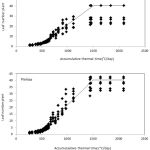Figure 1: The leaf production trend per plant versus Accumulative temperature unit in wheat cultivars.   Click here to view figure

 

The amount of philocrone, which is referred to as the time-period between the emergence of healthy leaves in the plant, which is, in fact, unlike that of the leaf emergence rate, in Pishtaz, is equivalent to 32.21°C per day and in SW is equivalent to 34.6°C per day.

PLAPOW Estimation

The power Equision. was used to describe the allometric regulation between the number of leaves in the main stem and the leaf area of ​​the plant .¹⁵

PLA = PLACON. MSNN ^plapow

This Equision. was fitted for wheat cultivars. The confidence level of 95% showed that no significant difference was found between wheat cultivars in terms of PLAPOW value. The value of determination coefficient between 0.27 and 0.81 in different densities indicates that a good correlation is found between the leaf area per plant and the leaf number in different densities (Table 3). Figure 2 shows the linear reduction of PLAPOW coefficient relative to the reduction in density in both wheat cultivars. That , PLAPOW is defined as a function of the plant density. In the model for PLAPOW, at a density of 100 plants per square meter in Pishtaz and SW, the values ​​were 1.46 and 1.58 respectively.²¹ Also used a power equation (y = x^b) . For describing the leaf area in versus the number of nodes . Contemporary both are increasing in number in the main stem. Using this power equation, were able to compare the leaf area of ​​the plant as a function of the plastochrone index (the interval between the sequential emergences of mung bean leaves.¹⁸

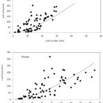Figure 2: The leaf area in the plant as a function of the number of leaves.   Click here to view figure

 

Table 3: The coefficient (b) of the equation PLA=MSNN^PLAPOW between the plant leaf area versus the number of nodes (or leaves) per plant in different plant densities, RMSE Root Mean Square Error and R² are determination Coefficients.

Cultivars	Density	b	RMSE	R2
Pishtaz	50	0.069 1.4994	61.71	0.2746
	100	0.048 1.4623	53.47	0.44
	150	0.034  1.4590	40.35	0.66
	200	0.039 1.4853	39.33	0.62
	300	0.0474 1.5499	39.31	0.5
	400	0.045  1.54499	35.55	0.55
SW	50	0.040  1.5499	63.8	0.62
	100	0.0264 1.58	43.61	0.81
	150	0.0343 1.5655	40.58	0.68
	200	0.045 1.5616	33.95	0.51
	300	0.057  1.6435	37.38	0.39
	400	0.063 1.6484	39.42	0.32

 

Estimated Light Extinction Factor (K)

K values are ​​calculated in this study for Pishtaz and SW cultivars .71 and .9 respectively.

Figure 3 shows the relationship between the radiation ratio and leaf area index in wheat cultivars (Pishtaz and SW) “R² is the coefficient of determination”.

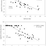Figure 3: Relationship between the radiation ratio and leaf area index in wheat cultivars (Pishtaz and SW) (R² is the coefficient of determination).   Click here to view figure

 

Estimation of Radiation Use Efficiency (RUE)

As shown in Fig. 4, the values ​​of the high determination coefficient indicate an appropriate relationship between accumulated dry matter and accumulated received radiation.²⁰ RUE value for Pishtaz was 2.36 g / mJ and 2.9 g / mJ for SW. According to a 95% confidence level, no significant difference was found between the two cultivars in terms of the efficiency of radiation use. RUE value for all cultivars was calculated to be 1.37 g / mJ (Fig. 5).

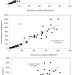Figure 4: Relationship between accumulated dry matter and accumulated received PAR in wheat cultivars (Pishtaz and SW and all cultivars).   Click here to view figure

 

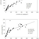Figure 5: The leaf dry matter as a function of total dry matter (both in grams per square meter) during the growing season to the seed growth stage in wheat (Pishtaz and SW) (RMSE, Root Mean Squared Error, and R² are Coefficients of Determination).   Click here to view figure

 

Figure 5 shows the relationship between accumulated dry matter and accumulated received PAR in wheat cultivars “Pishtaz and SW and all cultivars”.

The base temperature for dry matter production, the desired lower temperature for dry matter production, the upper limit of the desired temperature for dry matter production, and the ceiling temperature for the production of dry matter, based on available sources, are 10, 20, 30, and 40°C respectively(8).

Estimation of Dry Matter Distribution Parameters

The distribution of dry matter means the distribution of photosynthetic materials in different plant organs.²² To obtain the distribution parameters of dry matter before the end of the leaf growth on wheat cultivars, the data of the leaf dry matter were fitted against the total dry matter(9).

Y = x if  x< x_o

Y = b₁ x b₂ if x > x_o                                (2)

where y is the total dry weight, x is dry matter of the leaf or stem, x0 is the cycle point between two dry matter distribution stages (WTOPL), b1 is the distribution coefficient during the first stage (FLIF1A), and b2 is the distribution coefficient during the second stage (FLF2B). Figure 5 shows the fitting of two-part regression for obtaining FLF1A, FEF1B, and WTOPL coefficients in the cultivars studied for wheat in this study. As can be seen, at lower levels of the total dry matter (WTOPL), a greater part of the dry matter is allocated to the leaves (the first stage), but at higher levels of the total dry matter, lower dry matter is allocated to the leaves (the second stage). The allocation coefficients for the leaf in the first (FLIF1A) and the second (FLIF1B) parts in Pishtaz were .96 and .23 respectively, and, in SW, were .95 and .12 respectively. The cycle point from the first to the second part in Pishtaz and SW was 76.48 and 93.24 grams per square meter respectively. Therefore, when the accumulated dry matter content (WTOP) reaches 76.48 g / m² in Pishtaz and 93.24 g / m² in SW, FLF changes from FLF1A to FLF1B. With regard to the confidence level, a significant difference was found between the densities and cultivars in terms of the value of FLF1A WTPOL coefficient between two cultivars.¹⁵ The leaves have a higher concentration of nitrogen than the stems, and the maximum rate of nitrogen accumulation in Wheat  has an upper limit (ceiling).

The values ​​used in the model for FLF1A, FLF2B, and WTOPL were determined for Pishtaz and SW cultivars, based on the data obtained.

Non-independent evaluation of the model

Conventionally, the model is evaluated by comparing the outputs simulated by the model with real-world data gathered.²³  After estimating the plant parameters of SSM model in the previous section, the experiments performed to estimate parameters (Table 4) were simulated, and the output of the model was compared with the observed points (non-independent evaluation). The begining of this section is to determine the extent to which the model predictions are consistent with the measurements. If the predictions based on predefined criteria are in agreement with the measurements, the accuracy of the parameters’ estimation is confirmed, and then the model can be independently evaluated. For non-independent evaluation of the model, days to pollination and treatment, leaf area in pollination, number of leaves per main stem, dry weight in pollination, treatment and observed yield were compared with the simulation values by the model. Also, to test the results of the model, the evaluation indices, root mean square error (RMSE), coefficient of variation (CV), correlation coefficient (R), and the rate of deviation of the predicted results from 1:1 and ±18% lines were used.²⁴

Table 4: Specifications of the tests used to estimate the parameters and SSM-WHEAT model evaluation.

The experiment time and place in pakdasht	Treatment	Source
2015 -2016	Cultivar and planting date	(Nasrin mohammadi, 2016)
2013 -2014	Cultivar and planting date	Rajabi
2012 -2013	Cultivar and planting date	Rahimian et al.,
2012 -2013	Cultivar and planting date	Hejazi et al.,
2011 -2012	Cultivar and planting date	Akbari et al.,
2010 -2011	Cultivar and planting date	Akbari et al.,

 

The results of the phonological evaluation of the model showed that the root mean square error (RMSE) for the day to pollination was 61.51 days. The simulated and observed coefficient of variation (CV) was equal to 21.18, which indicates the high accuracy of the model for the prediction of phonological stages. Also, the high correlation between the simulated and observed phenology shows that the model has been successful in predicting the phenology (Fig. 6).

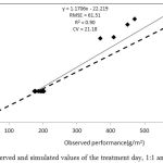Figure 6: Observed and simulated values of the treatment day, 1:1 and +18% lines.   Click here to view figure

 

The model was evaluated by using the cultivars Mahdavi, Narin, Pishgam, Zagros, Pishtaz, and Sirvan which were tested in previouse years in the same condition and the results of leaf area (m² / m²) LAI, fraction of available water FASW, accumulated crown dry weight (g / m²) WTOP, accumulated seed dry weight (grams per square meter) WGRN, seed growth rate (grams per square meter per day) SGR, product growth rate (grams per square meter per day) DBP, daily transpiration (mm / day) TR were shown graphically. The cultivar Pishtaz—common to the Pakdasht area—is described as an example.

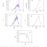Figure 7: Evaluation of the cultivar Pishtaz. A. SGR: Seed growth rate; B. TR: Daily transpiration; C. LAI : Leaf area; D. WTOP: Accumulated crown dry weight. E. FASW: fraction of available water.   Click here to view figure

 

The model was evaluated using the cultivars Mahdavi, Narin, Pishgam, Zagros, Pishtaz and Sirvan and the results of leaf area (m² / m²) LAI, fraction of available water FASW, accumulated crown dry weight (g / m²) WTOP, accumulated seed dry weight (grams per square meter) WGRN, seed growth rate (grams per square meter per day) SGR, product growth rate (grams per square meter per day) DBP, daily transpiration (mm / day) TR were shown graphically. The cultivar Pishtaz- common to the Pakdasht area, is described as an example.

Figure 8: Model Application a:   Click here to view figure

 

The minimum temperature is increasing by 0.03 slope per year; b: The maximum temperature is increasing by .05 per year; c: The average temperature is increasing by 0.04 per year; d: The rainfall is reducing by -0.8 annually; e: The maximum leaf area index is 0.007; f: The plant growth per year is 5.9; g: Cumulative dry weight of the grains is increasing by 2.5 per year.

The model application

Parameterization of Tmin, Tmax, Tmean, WVEG, WGRN, Rain, Maxlai, and DTBSG-DTHAR by SSM model for the analysis of wheat growth and yield potential under Tehran conditions from 1983 to 2015. These parameters show us that how the model works in comparison with another situation.

The minimum temperature is increasing by 0.03 slope per year.

The maximum temperature is increasing by .05 per year.

The average temperature is increasing by 0.04 per year.

The rainfall is reducing by -0.8 annually.

The maximum leaf area index is 0.007.

The plant growth per year is 5.9.

Cumulative dry weight of the grains is increasing by 7.1 per yea.

Conclusion

In this research, the wheat model (SSM) was used. This model has open source and, because it has a simple structure, can also be used for educational purposes. Since the model uses Excel for input and output, it is easy to work with. This model can be used in many cases, including research applications; crop management and education are examples of this. In this research, the required parameters of SSM model in the phonologic development, production and distribution of dry matter, leaf area growth and decay, yield using field experiment as well as available resources in other researches for wheat, (two cultivars of Pishtaz and SW) were prepared and used in the model. By using them, parameters were estimated, simulation was performed, and the output of the model was compared with the observed points (non-independent evaluation). Non-independent evaluation results, leaf area index, and number of nodes per plant, biomass, and yield showed that the model has an acceptable predictive power for the plant.

According to Tehran’s meteorological data, which was used in the model from 1983 to 2015, the results are based on this principle that with the increase in maximum temperature – minimum temperature – average temperature and annual precipitation, the number of days required to reach each stage of the plant phenology has been reduced, which is reasonable.

References

1. Rötter R., Tao F., Höhn J., Palosuo T. Use of crop simulation modelling to aid ideotype design of future cereal cultivars. Journal of experimental botany. 2015;66(12):3463-76.
   CrossRef
2. Baez-Gonzalez A. D., Kiniry J. R., Meki M. N., Williams J., Alvarez-Cilva M., Ramos-Gonzalez J. L., et al. Crop Parameters for Modeling Sugarcane under Rainfed Conditions in Mexico. Sustainability. 2017;9(8):1337.
   CrossRef
3. Mamone G., Caro S. D., Luccia A. D., Addeo F., Ferranti P. Proteomic‐based analytical approach for the characterization of glutenin subunits in durum wheat. Journal of Mass Spectrometry. 2009;44(12):1709-23.
   CrossRef
4. Ritchie J., Singh U., Godwin D., Bowen W. Cereal growth, development and yield. Understanding options for agricultural production: Springer. 1998;79-98.
   CrossRef
5. Shani U., Ben‐Gal A., Tripler E., Dudley L. M. Plant response to the soil environment: An analytical model integrating yield, water, soil type and salinity. Water resources research. 2007;43(8).
   CrossRef
6. Hoogenboom G., White J. W., Messina C. D. From genome to crop: integration through simulation modeling. Field Crops Research. 2004;90(1):145-63.
   CrossRef
7. Whisler F., Acock B., Baker D., Fye R., Hodges H., Lambert J., et al. Crop simulation models in agronomic systems. Advances in agronomy. 40: Elsevier. 1986;141-208.
8. Soltani A. Modeling physiology of crop development, growth and yield: CABi. 2012.
9. Sinclair T., Farias J., Neumaier N., Nepomuceno A. Modeling nitrogen accumulation and use by soybean. Field Crops Research. 2003;81(2-3):149-58.
   CrossRef
10. Robertson M., Asseng S., Kirkegaard J., Wratten N., Holland J., Watkinson A., et al. Environmental and genotypic control of time to flowering in canola and Indian mustard. Australian Journal of Agricultural Research. 2002;53(7):793-809.
    CrossRef
11. Fehr W. R., Caviness C. E. Stages of soybean development. 1977.
12. Wilhelm J. E., Mansfield J., Hom-Booher N., Wang S., Turck C. W., Hazelrigg T., et al. Isolation of a ribonucleoprotein complex involved in mRNA localization in Drosophila oocytes. The Journal of cell biology. 2000;148(3):427-40.
    CrossRef
13. Soltani A., Sinclair T.R. A simple model for chickpea development, growth and yield. Field Crops Research. 2011;124(2):252-60.
    CrossRef
14. Soltani A., Sinclair T. R. A comparison of four wheat models with respect to robustness and transparency: simulation in a temperate, sub-humid environment. Field Crops Research. 2015;175:37-46.
    CrossRef
15. Soltani A., Robertson M., Mohammad-Nejad Y., Rahemi-Karizaki A. Modeling chickpea growth and development: Leaf production and senescence. Field crops research. 2006;99(1):14-23.
    CrossRef
16. Boote K., Pickering N. Modeling photosynthesis of row crop canopies. Hort. Science. 1994;29(12):1423-34.
17. Sinclair T. R. A reminder of the limitations in using Beer’s law to estimate daily radiation interception by vegetation. Crop science. 2006;46(6):2343-7.
    CrossRef
18. Soltani A., Torabi B., Zarei H. Modeling crop yield using a modified harvest index-based approach: application in chickpea. Field crops research. 2005;91(2-3):273-85.
    CrossRef
19. Bindi M., Sinclair T., Harrison J. Analysis of seed growth by linear increase in harvest index. Crop Science. 1999;39(2):486-93.
    CrossRef
20. Soltani A., Khooie F., Ghassemi-Golezani K., Moghaddam M. Thresholds for chickpea leaf expansion and transpiration response to soil water deficit. Field Crops Research. 2000;68(3):205-10.
    CrossRef
21. Hammer G., Carberry P., Muchow R. Modelling genotypic and environmental control of leaf area dynamics in grain sorghum. I. Whole plant level. Field Crops Research. 1993;33(3):293-310.
    CrossRef
22. Vries F. P. d. Simulation of ecophysiological processes of growth in several annual crops: Int. Rice Res. Inst. 1989.
23. Reynolds J. F., Acock B. Modularity and genericness in plant and ecosystem models. Ecological modelling. 1997;94(1):7-16.
    CrossRef
24. Soltani A., Hoogenboom G. Assessing crop management options with crop simulation models based on generated weather data. Field Crops Research. 2007;103(3):198-207.
    CrossRef

(Visited 493 times, 1 visits today)