Jan Thomas, Vinupritha P and Kathirvelu D

Department of Biomedical Engineering, SRM University, Kattankulathur–603 203, Tamilnadu, India.

Corresponding Author E-mail: vinupritha@gmail.com

DOI : https://dx.doi.org/10.13005/bpj/1183

Abstract

The central nervous system (CNS) directs a large number of muscles to produce complex motor behavior’s. Moreover, human movement control is significantly compromised in neuromuscular diseases; many of which result from the imbalance in the sensorimotor control system. Forward models are also known to capture the casual relationship between the inputs to the system and its output. The aim of this study was to approximate a forward dynamic simulation by using feed forward neural networks in human elbow arm movement. Motion capture data was used to generate c3d data from Qualisys software via Qualisys track manager. The c3d data was then converted into marker data which contains the markers location in the form of x-y-z coordinate. OpenSim- biomechanical software was used to process the marker data for scaling, inverse kinematics and the subsequent forward dynamics simulation in the right human upper arm model. The results for the training error of the approximated forward dynamics simulation for 3 degrees of freedom (DOF) were 2.804429, 1.468017 and   2.475500 with a constant validation error of 0.000000. The proposed control algorithm served as robust method for approximating a forward dynamic simulation, and can broaden the understanding the representations of neuromuscular control in the central nervous system as representations of movement plans that are eventually executed by the spinal cord and muscles in the periphery.

Keywords

Neural networks; Open Sim; Forward dynamics; CNS

Download this article as: 

Copy the following to cite this article: Thomas J, Vinupritha P, and Kathirvelu D. Neuromuscular Control with Forward Dynamic Approximation in Human Arm. Biomed Pharmacol J 2017;10(2).

Copy the following to cite this URL: Thomas J, Vinupritha P, and Kathirvelu D. Neuromuscular Control with Forward Dynamic Approximation in Human Arm. Biomed Pharmacol J 2017;10(2). Available from: http://biomedpharmajournal.org/?p=14930

Introduction

Human movement control is significantly compromised in neuromuscular diseases; many of which result from the imbalance in the sensorimotor control system. Muscle excitation that follows the neural impulses to generate movements common in daily activities like reaching, grasping holding plays a key role in the mechanism of motion from the sensory input [1,2]. Neural Networks have also gained popularity in their usage in fields such as Natural Language Processing, Computer Vision, reinforcement learning, and even animation [3,4]. The primary motivation of this study was similar previous studies which discuss the control of multijoint movements by the CNS to perform complicated transformations from the desired behavioral goals into appropriate neural commands to muscles [5]. A model thus formulated was proposed by defining an objective function, which is considered as a performance measure for any possible movement: square of the rate of change of torque integrated over the entire movement [6-8]. Furthermore, many studies have also discussed the use of neural network model was developed to understand the internal organization of movement generation [9-11]. The use of recurrent neural networks is discussed in detail where recurrent neural network is trained to produce the muscle activity of the reaching monkeys resulting in a dynamics where  simple inputs were transformed  into temporally and spatially complex patterns of muscle activity [12] .Past researches in the field of motor control have also discussed the criterion that is adopted for determination of the trajectory wherein the common invariant features were found in several researches that measured the hand trajectories of skilled movements[13]. The hand movement for instance, between a pair of targets, subjects tended to generate roughly straight hand paths with bell-shaped speed profiles. These observations along with dynamic optimization theory, led to the design of a mathematical model which accounts for formation of hand trajectories [13,5] .The use of neural networks which contains internal model of inverse dynamics as essential learning parts of the musculoskeletal system was the main feature in the learning of voluntary motor control [14]. Other studies emphasize the forward model as representation of motor system that predicts the next state using the current state of motor system and motor commands [15].

This study will discuss its application to approximating and controlling muscle activation with feed forward neural networks. The only goal of this study is to see if we could achieve values using the above strategy in order to have a broader understanding as to how neural signals of the motor cortex relate to movement. We have selected a musculoskeletal model that we will use for our neural network approximation. In order to achieve our goal, we generate forearm flexion movements in an allowable range in order to train and test our neural network.

Materials

OpenSim

OpenSim is a software framework designed to build and share musculoskeletal models, simulate movements, and analyze and visualize those movements using specialized tools. This framework contains, amongst other things, a graphical user interface (GUI) scripted in java language, various built-in musculoskeletal models developed and published by an open source community of researchers and users, a software development kit, APIs and other various tools that are used by researchers or hobbyists for analysis [16]. OpenSim has many open source musculoskeletal models available in their repository. These include human and animal models that can vary in complexity and scope. In this study, we are only looking at the right arm of a human which consists of 2 degrees of freedom, with 6 muscles and   muscle elements such as bones, ligaments, etc. and provides a dynamic graphical simulation to visualize and analyze moments about the joints of a human arm [16]. There are multiple arm models that are available and we have the liberty of choosing one that we believe can achieve our objective simply and effectively. There are many tools available on the platform that can be used to analyze muscle actuation and joint position. We use an arm model whose muscles are based on Hill’s muscle model [16,17] , which is shown in fig 1.

Motion Capture System

The motion capture device used for this study was Qualisys motion capture system (Qualisys Inc) with Qualisys Track Manager (QTM) allows users to perform 2D, 3D and 6DOF capture of data in real-time by the way of C3D data which is then converted into in a .trc file which provides the distances between markers on the model and experimental marker positions which are compared and determined by the scaling factors [6]. For this study the scaling factor was set to 1.0 which is the default scaling factor used in OpenSim software. The experimental markers set for 15 healthy subjects were right acromium; right humerus epicondyle and right styloid process of radius to match with the generic marker in model. The unscaled model should have a set of virtual markers placed in the same anatomical locations as the experimental markers. The modeling of the neural network architecture was carried out in Matlab 2013 platform. Matlab is a high level language and interactive environment for numerical computation, visualization and programming. MATLAB provides a range of numerical computation methods for analyzing data, developing algorithms, and creating models .The inverse and forward simulation along with the conversion of motion capture data were performed via Matlab-OpenSim interface [18,19].

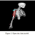Figure 1: Open sim Arm model   Click here to View figure

Scaling

Scaling is performed based on a combination of measured distances between x-y-z marker locations which were obtained from the data specified in the track row column (trc) files and manually-specified scale factors. The marker locations are usually obtained using motion capture equipment. For pair 1 on the model (m1) the distance is computed by placing the model as all joint angles get assigned their default values. The experimental distance between pair 1 (e1) is computed by looking at each frame of experimental marker data in the given .trc file, computing the distance between the pair for that frame, and taking the average across all frames in a user-specified time range. The scale factor due to pair is s1=e1/m1.

Methods

The schematic of the proposed approach to perform neuromuscular control with forward dynamic approximation is shown in Fig.2

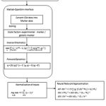Figure 2: Schematic of the work flow   Click here to View figure

Inverse kinematics

The Inverse Kinematics (IK) tool computes generalized coordinate values which positions the model in a pose. This pose “best matches” experimental marker and coordinate values for that time step or the frame of motion [1,15] .Mathematically, the “best match” is expressed as a weighted least squares problem, whose solution minimizes both marker and coordinate errors. The marker error is the distance between an experimental marker and the corresponding generic marker on the model; the IK solver computes the generalized coordinates and is used to position the markers. Each marker has a weight associated with it, which specifies the extent to which that marker’s error term should be minimized. The IK solver is given by the following equation as the weighted least squares problem solved by IK.

min [∑ w_i || x_i^exp – x_i (q) ||² + ∑ ɷj(q_j^exp– q_j) ² ]                                   (1)

^{q       iϵ markers                                j ϵ unprescribed coords}

where q is the vector of generalized coordinates being solved for, x_i^exp is the experimental position of marker i, x_i (q) is the position of the corresponding marker on the model (which depends on the coordinate values), q_j^exp is the experimental value for coordinate j. The marker weights (w_i‘s) and coordinate weights (ω_j‘s). This least squares problem is solved using a general quadratic programming solver, with a convergence criterion of 0.0001 and a limit of 1000 iterations.

This generates motion file with the times histories of joint angles [1] shown in table 1.

Table 1: A motion data containing time histories of joint angles in degrees.

Time	Joint 0	Joint 1	Joint n
t0	θ00	θ01	θ02
t1	θ10	θ11	θ12
t2	θ 20	θ21	θ 22
tm	θm1	θm2	θ m3

Each of the positions are in units of radians. For our model, we have 2 Degrees of Freedom (joint angles) that correspond to 2 joints, namely glenohumeral (GH) and elbow (EL). Each joint has a minimum and maximum value for position expressed as radians.

Forward dynamics

The Forward Dynamics Tool can drive a forward dynamic simulation. A forward dynamics simulation is the solution (integration) of the differential equations that define the dynamics of a musculoskeletal model [1,18]. By focusing on specific time intervals of interest, and by using different analyses, more detailed biomechanical data for the trial in question can be collected. From Newton’s second law, accelerations (rate of change of velocities) of the coordinates can be described in terms of the inertia and application of forces on the skeleton as a set of rigid-bodies: This is given by the following equation

q̈ = [M (q)]^-1{τ + C (q, q̇) + G (q) +F}                                                      (2)

Where q̈ is the coordinate accelerations due to joint torques τ Coriolis and centrifugal forces, C(q,q̇) as a function of coordinates q ,and their velocities q̇, gravity G(q), and other forces applied to the model F, and M[(q)]^-1  is the inverse of the mass matrix. The state of a model is the collection of all model variables defined at a given instant in time that are governed by dynamics. The model dynamics describe how the model will advance from a given state to another through time. In a musculoskeletal model the states are the coordinates and their velocities and muscle activations and muscle fiber lengths. The dynamics of a model require the state to be known in order to calculate the rate of change of the model states (joint accelerations, activation rates, and fiber velocities) in response to forces and controls [1]. This generates the controls file which gives the time histories of muscle excitations shown in table 2.

Table 2: A controls data containing time histories excitation patters of biceps   long and short head muscles

Time	Biceps_long head	Biceps_short head
t1	Excitation11	Excitation 13
t2	Excitation 21	Excitation 23
t3	Excitation 31	Excitation 33
t4	Excitation 41	Excitation 43
t5	Excitation 51	Excitation 53
t6	Excitation 61	Excitation 63

Neural Network Architecture

Neural Network architecture is imbibed from the computational phenomenon of the brain. In the brain neurons are connected to each other and fire when the sufficiently appropriate stimuli are presented. Inputs gathered by the Neuron and then passed through an activation function which produces an output from the neuron. These outputs are then propagated throughout the neural network and in the final stage, combined into an output value used to interpret the relevant state of the application shown in fig 3.

Figure 3a: Neuron (b) Network configuration [*Green dots represent connected neurons in each layer]   Click here to View figure

Neurons are arranged in layers labeled as input, hidden, or output. Input layers represent the inputs to the neural network. The hidden layers are between the inputs and outputs. The output layer is the observable. Each neuron in layer l receives weighted inputs from layer l-1and sums them together along with a bias before passing them through activation function. The bias shifts the input sums along the sigmoid function and can be beneficial to biasing the output towards a particular value. The activation function may change depending on the situation of the neural network, but typically it is the sigmoid function expressed in eq (3) and shown in fig 4.

g(z) = 1/(1+e^-z)                                                    (3)

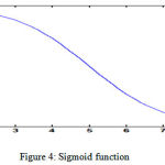Figure 4: Sigmoid function   Click here to View figure

Feed forward network with 1 input layer, 3 hidden layers, and a single output layer was used. It was fully connected such that each neuron in the previous layer is connected to all neurons in the next layer. Each hidden layer size is the same as the number of inputs created at the beginning of the network shown in fig 5.

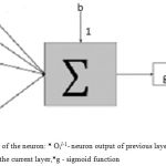Figure 5: Architecture of the neuron: * Oil-1– neuron output of previous layer,*W and b- the weights and biases of the current layer,*g – sigmoid function   Click here to View figure

Sampling

The sampling required motion kinematics data (.mot file) and state data in storage (Controls.sto) file. The states file can contain the time histories of model states, including joint angles, joint speeds, muscle activations, muscle fiber lengths, and more. The forward dynamics Tool to set the initial states of the model for forward integration. Muscle states can be estimated by solving for tendon and muscle fiber force equilibrium when the solution for equilibrium for actuator states is checked. The control data contains the time histories of the model controls (e.g., muscle excitations) to the muscles and/or joint torques, for this study biceps long head and short head was considered. It is possible to specify the controls as .sto files instead, with columns corresponding to desired excitations.

Normalisation

The inputs and the outputs were normalized between 0 and 1 by using the following equation

êj= ej – min(Ci)/max(Ci) – min(Ci)                             (4)

Ci is the i^th degrees of freedom. The max and min are the maximum values and minimum values of the degree of freedom, ej and is the j^th element.

Initialisation

Initialization of the network was done with 13 random inputs each with 12 dimensions which correspond to the down sample rate of 3 for 100 time steps. The network has 5 layers where the first and the last are input and output layers, leaving 3 hidden layers. There are 50 training rounds in each of the 50 epochs. The neural network was tested by down sampling the motion files and controls file by a factor k = 3. This decreases the amount of neurons used for our network and significantly lowers the amount of time needed for training and testing. The training consists of each input which is a 1X3 vector which represents the state at some time step. Each weight is multiplied elemental wise with the input and subsequently summed together column-wise. The bias is then added to the result and then each element of the new vector is passed through the sigmoid function.

Training

The training involved modified back propagation algorithm along with stochastic gradient descent [10]. The error function is expressed in equation 5

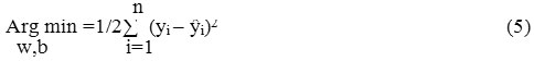
Where y_i is the associated true output and ŷ_i is the predicted output from the neural network. The weights and biases of the network are represented by w and b. We sum across all the outputs of our network to gather all the contributing errors. By finding the gradients with respect to each parameter, we will then update each parameter by taking a step in the direction of the gradient to decrease this error function. The weights and biases are updated in the direction of the negative gradient of the performance function.

The algorithm for training is as follows: A random training example from training pool is chosen. Pass training input through the network and determine objective loss

for

Calculate each nodes in output layer by

Computing gradients with respect to biases

Computing gradients with respect to weights

Computing gradients with respect to previous layer

end for (Calculate gradients with respect to outputs backwards through the layers)

Repeat using output gradients from the next layer for:

Computing gradients with respect to biases

Computing gradients with respect to weights

Computing gradients with respect to previous layer until    input layer is reached

for

Update all weights and biases based on the computed gradients by a step size

end for

For each neuron output:

O^l_{j =} g (Ʃ (O_i^l-1W_ij^l) + b_j                                                   (6)

g is the sigmoid activation function. O^l_j is the output of node j in layer l where O_i^l-1 is the output from the previous layer and W and b are the weights and biases of the current layer respectively.

The gradients for weight, biases and previous output are as follows:

∂O^l_j  ∕ ∂W_ij^l = g^ʹ (Ʃ (O_i^l-1W_ij^l) + b_j^l) O_i^l-1                              (7)

O_i^l-1 contributes to all of the outputs in the next layer and so in order to back propagate the contribution, we have to average all of its contributions as follows:

∂O^l/ ∂O_l^l-1 = 1/N ∑ (g^ʹ (Ʃ (O_i^l-1W_ij^l) + b_j^l) W_ij^l                  (8)

∂O_l^j ∕ ∂ W_ij^l-1 = ∂O_l^j/∂O_l-1 * O_l-1/ W_ij^l-1                              (9)

∂O_l^j ∕ ∂ b^l-1 = ∂O_l^j/∂O_l-1 * O_l-1/ b^l-1                                  (10)

The chain rule is applied to find the gradients with respect to the weights and biases of previous layers using the above equations. Once the gradients have been calculated, the weights were updated update each weight element by a step size into the gradient direction. The step size in the current study is 0.5 since the gradients were small compared to actual weights. This is probably due to the fact that normalization required each weight and input to be between 0 and 1 and thus these values will be multiplied together during training to result in a very small value. Therefore a step size large enough to influence the objective error function in each epoch was used.

Validation

In this study, 15 samples operating on 15 training examples for each of the 20 epochs were presented to the network. The network selects 95% of the data for training leaving 5% for validation The data produced by forward dynamics simulation from the 15 samples were validated. The network updates the weights and biases and uses those updated parameters for the validation set through training and is shown in fig 6.

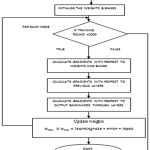Figure 6: Schematic of the training algorithm   Click here to View figure

Results and Discussion

Results of Inverse Kinematics simulation is shown in table 3

Table 3: Kinematics data in degrees:*r_shoulder_elev- right shoulder elevation,* r_elbow_flex -right elbow flexion.

Time	r_ shoulder_elev	r_elbow_ flex
0.000000	-0.03349	-0.05440
0.008333	-0.03657	0.014179
0.016667	-0.03908	0.088157
0.025000	-0.04126	0.173575
0.033333	-0.04317	0.275760
0.041666	-0.04510	0.399452
0.050000	-0.04512	0.548699
0.066667	-0.04434	0.726772
1.00000	-0.03549	90.170666

Results of Forward Dynamics simulation is shown in table 4

Table 4: State data of muscle excitation:*Biceps LH- Biceps long head, *Biceps SH- Biceps short head.

Time	Biceps LH	Biceps SH
0.00000002	0.01007429	0.01028343
0.00000004	0.01007438	0.01028345
0.00000006	0.01007445	0.01028365
0.00000006	0.01007467	0.01028388
0.00000008	0.01007470	0.01028398
0.00000011	0.01007476	0.01028376
0.00000016	0.01007485	0.01028355
0.00000025	0.01007489	0.01028389
0.00000039	0.01007494	0.01028353
0.99999994	0.01000356	0.18449298

Results of Baseline testing of the neural network is shown in fig 7

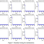Figure 7: Baseline testing for initialization   Click here to View figure

Results of training and validation error shown in table 5 and fig 8 and 9

Table 5: Results of training and validation error

Degrees of freedom	1	2	3
Training error	2.804429	1.468017	2.475500
Validation error	0.000000	0.000000	0.000000

 

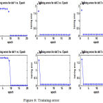Figure 8: Training error   Click here to View figure

 

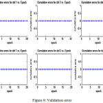Figure 9: Validation error   Click here to View figure

In the past several models were developed to understand motor control in human that is incorporated in designing the robotic system. At present there are various models that use recurrent neural network along with supervised learning. A study by Kawato et al proposed, proposed a mathematical model which accounts for formation of hand trajectories. This model is formulated by defining an objective function, a measure of performance for any possible movement. This objective function is determined complex nonlinear dynamics of the musculoskeletal system square of the rate of change of torque integrated over the entire movement. This study was done in an effort to understand the trajectory planning and control of voluntary human movements[6,9].

A more recent study on reaching tasks in monkeys was carried out by Susillo et al concluded the solution generated by recurrent neural network which was a low dimensional oscillator resulting in multiphasic commands; in order to understand the dynamics that transformed simple inputs into both  spatially and temporally complex muscle activity[11]. The study by  Jordan et al, demonstrated that certain classical problems associated with the notion of the “teacher” in supervised learning con be solved by judicious use of learned internal models as components of the adaptive system[10]. In particular it focused on how supervised learning algorithms can be utilized in cases in which an unknown dynamical system intervenes between actions and desired outcomes. Thus in the light of previous studies, the present study proposes a control algorithm based on feed forward that uses stochastic gradient descent to compute the errors for learning strategy. The study executes a forward dynamics simulation approximated by the feed forward neural network, in an attempt to understand the inputs from the CNS that are transformed into movements by the way of synergistic muscle activities. The network only updates the weights and biases through training and uses those updated parameters for the validation set. The validation graphs reflect the training error graphs in their behavior. The degree of freedom which represents the time index shows graph where the output times and input times are similar and that this error is the lowest error of all the degrees of freedom as would be expected.Further in the results it is seen that the validation error follows a similar pattern as the training error, suggesting the possibility approximating the forward simulation. This would indicate that forward dynamics simulation can be approximated by a neural network. It also important to considered the relatively small sample size used for the study as a limitation which resulted in similar patterns of the cumulative errors throughout the epochs. A larger sample size could have shown more pronounced results with regard to the changes in the errors values for the corresponding training errors with greater computational costs. Moreover, the study was circumscribed by the constraints in the degrees of freedom which limited the movements to elbow flexion in allowable range. The activities of the secondary muscles that aid in elbow flexion were consequently beyond the scope of this study.

Conclusion

A common cumulative error was achieved that corresponded to the training errors in order to approximate the simulation of forward dynamics. Hence it can be concluded that control algorithm that uses feed forward neural network along with back propogation by gradient descent is a robust method in an effort to mimic the execution and motor planning of the brain when performing simple tasks. Furthermore, the proposed control algorithm can be judiciously used with both supervised and unsupervised learning algorithms.

Acknowledgements

The authors wish to express their deep sense of gratitude to the co-workers for their constant support throughout the study.

References

1. Emel Demircan, Oussama Khatib, Scott delp.Reconstruction and EMG-Informed Control Simulation Analysis of Human Movement For Athletes:Improvement and Injury Prevention. Conf Proc IEEE Eng Med Biol Soc.September 2015.
2. Demircan E, Sentis L, De Sapio V, Khatib O. Human Motion Reconstruction by Direct Control of Marker Trajectories. In: Lenarcic J, Wenger P, editors. Advances in Robot Kinematis.2008.,Springer Netherlands, pp. 263–272.
   CrossRef
3. Radek Grzeszczuk, Demetri Terzopoulos, and Geoffrey Hinton. Neuroanimator:Fast neural network emulation and control of physics-based models. In Proceedings of the 25th Annual Conference on ComputerGraphics and Interactive Techniques, SIGGRAPH .1998., pages 9–20, New York, NY, USA.
4. Paul J. Webros.Backpropogation Through Time: What it does and How to do it. Proceedings of the IEEE.1999., Vol 10.
5. Tamar Flash, Michael.J Jordan.Computational schemes and neural networks model of human arm trajectory control. World congress of neural networks.1999., pp.76-83.
6. Mitsuo Kawato.Formation and Control of Optimal Trajectory in Human Multijoint Arm Movement. Cybernetics.1989., Vol 61, pp 80-89.
7. Tamar Flash, Terrence J Sejnowski.’Computational approaches to motor control.Trends Cogn Sci.1997.,Vol 1, pp209-16.
   CrossRef
8. Schweighofer N., Arbib M. A., Kawato M.Role of the cerebellum in reaching movements in humans in Distributed inverse dynamics control. J. Neurosci.1998., Vol 10, pp 86–94.
9. Kawato M1, Furukawa K, Suzuki R.A hierarchical neural-network model for control and learning of voluntary movement.Biol Cybern.1987., Vol 3,pp 169-85.
10. Jordan MI, Rumelhart DE. Forward models – supervised learning with a distal teacher. Cogn Sci .1992., Vol 6,pp 307-54.
    CrossRef
11. David Sussillo, Mark M Churchland, Matthew T Kaufman & Krishna V Shenoy et al.A neural network that finds a naturalistic solution for the production of muscle activity.Nature Neuroscience.2015., volume 18.
    CrossRef
12. Nikhil Bhushan and Reza Shadmehr. Evidence for a Forward Dynamics Model in Human Adaptive Motor Control. Advances in Neural Information Processing System1999.,Vol. 11, pp. 3-9.
13. Hogan N., Bizzi E., Mussa-Ivaldi F. A., Flash T. Controlling multijoint motor behavior. Sport Sci.1987., Rev, Vol 15, pp153–190.
14. M. Wolpert, M. Kawato.Multiple paired forward and inverse models for motor control .Neural Networks.1998., Vol 11, pp 1317–1329.
    CrossRef
15. C MIall, D.M Wolpert.Forward models for physiological motor control. Neural Networks. 1996.,Vol.9, Number 8, pp 1265-1279.
    CrossRef
16. Scott L. Delp, Frank C. Anderson, Allison S. Arnold, Peter Loan, Ayman Habib, Chand T. John,Eran Guendelman, and Darryl G. Thelen et al.OpenSim: Open-Source Software to Create and Analyze Dynamic Simulations of Movement .IEEE Transactions on biomedical engineering.,vol. 54, Number 11.
    CrossRef
17. Thelen DG, Anderson FC, Delp SL. Generating dynamic simulations of movement using computed muscle control. Journal of Biomechanics.2003., No.36, pp 321–328.
    CrossRef
18. Mantoan,C,Pizzolato,M.Sartori,Z.Sawacha,C.Cobelli,M.Regianni.MOtoNMS: A Matlab toolbox to process motion data for neuromusculoskeletal modeling and simulation. Source code for Biology and Medicine. ,pp 44.
19. Khatib O, Brock O, Chang K, Conti F, Ruspini D, Sentis L. Robotics and Interactive Simulation. Communications of the ACM.2002., Vol 3, pp 46–51.
    CrossRef

(Visited 957 times, 2 visits today)