Sumit Kushwaha and Rabindra Kumar Singh

Electronics Engineering Department, Kamla Nehru Institute of Technology, Sultanpur, India.

Corresponding Author E-mail: sumit.kushwaha1@gmail.com

DOI : https://dx.doi.org/10.13005/bpj/1171

Abstract

Medical imaging is an indispensable tool for diagnosis of several complex disorders. In preceding years, advancement in medical imaging have aided in accurate diagnosis by capturing the anatomical images of the human organs without the necessity to surgically treat the human body. A radical medical diagnosis requires accurate results from the imaging modalities that are generally vulnerable to noises, resulting in a blemished image. In case of ultrasounds, the major noise is the speckle noise. Several tissues in the human body are hard that are accountable for producing multiple reflections of the ultrasound waves causing speckle noise which vitiates the quality of the ultrasound images. We present an efficient denoising method for the ultrasound images that will overcome the noising, particularly obtained through speckle noise. This paper adopts Anisotropic Diffusion for denoising of the image. This paper provides additionally the performance analysis of the denoising mechanism using the Teaching-Learning Based Optimization methods to achieve the targeted results. Also, HSOA algorithm is used for this purpose and the results from both the techniques are compared. The technique for denoising proposed in this paper has extensively enhanced the denoising mechanism used in ultrasound images of the liver. While the proposed system is considered to be effective, however the performance of the denoising carried out by the TLBO algorithm concluded that the denoising was over-filtering the image with the additional loss of data.

Keywords

Ultrasound image; Denoising; Anisotropic Diffusion; Teaching–learning based optimization (TLBO) algorithm; Harmony search optimisation algorithm (HSOA)

Download this article as: 

Copy the following to cite this article: Kushwaha S, Singh R. K. An Efficient Approach for Denoising Ultrasound Images using Anisotropic Diffusion and Teaching Learning Based Optimization. Biomed Pharmacol J 2017;10(2).

Copy the following to cite this URL: Kushwaha S, Singh R. K. An Efficient Approach for Denoising Ultrasound Images using Anisotropic Diffusion and Teaching Learning Based Optimization. Biomed Pharmacol J 2017;10(2). Available from: http://biomedpharmajournal.org/?p=14956

Introduction

Attributed to rapid development in technology, the medical field has substantially improved with successful diagnosis and effective treatment. Doctors are able to treat patients on the basis of various non-invasive imaging modalities including X-ray’s, Computed tomography, Magnetic Resonance Imaging (MRI), Ultrasound, Positron Emission Tomography (PET) and Single Photon Emission Computed Tomography (SPECT). Muscle imaging is significant in order to detect disorders of muscles. Muscle imaging is generally carried out by MRIs, CT scans and Ultrasound. A comparison of these imaging modalities is depicted in table 1. While capturing the images, there is some amount of noise and artifacts present in the image that may obscure the diagnosis by distorting the data and concealing various problems. Therefore, it is highly essential to denoise the images to obtain the accurate images [1]. It is however deduced from this table that ultrasound has many benefits relative to others and is ideal for imaging muscles. Therefore for this research, ultrasound imaging has been considered.

Table 1:  Comparison of muscle imaging modalities, adapted from Clague et al [2].

	Ultrasound	CT	MRI
Availability	Readily available	Readily available	Increasing
Relative cost	Inexpensive	Expensive	Very expensive
Portability	Portable	Fixed	Fixed
Muscle	Fair	Good	Very good
Repeatability	Yes	Limited	Yes
Safety	Non-ionizing	Ionizing radiation	Non-ionizing

Ultrasound makes use of ultrasonic waves that are generated from the transducer and pass over our body tissues. The waves that are coming back are sound waves that pulse the transducer. Finally, the waves convert into electrical pulses which are required to go to the ultrasonic scanner. The scanner is responsible for processing and converting the recorded data into a digital image [3]. While the image quality can be improved with greater frequencies, this restrains the intensity of the dispersion of the waves. Noising is common attributed to several factors such as technical errors, i.e. errors pertaining to the technique of capturing the ultrasound or processing errors pertaining with the errors occurring during processing [4]. Artifacts may perhaps arise consequently due to incorrect way of usage of the ultrasound machine, and accidents accompanying processing of the images, and from smaller defects in the image which is occasional. Similarly, too much movement or vibration of the ultrasound probe because of some defect, or the patient’s movement also may lead to artifacts.

An intrinsic attribute of ultrasound imaging is the presence of speckle noise. Ultrasound is commonly affected by speckle noise that reduces the delicate specifics and boundaries of the image besides constraining the image resolution to conceal the miniscule abrasions of an organ. Speckle noise is arbitrary and deterministic in an ultrasound image. The main requirement for enhancing the image quality is developing effective approaches that reduce the noise considerably without affecting the data to be perceived [5]. A huge amount of research has been undertaken to reduce the speckle noise such as temporal averaging homomorphic wiener filtering [6], median filtering [7], adaptive speckle reduction [8], wavelet thresholding [9] and the like. The adaptive filtering considers the image’s numerical characteristics and is contemplated to be an ideal technique for ‘despeckling’ the image [10][11][12]. Recently, non-linear Partial Differential Equations (PDE) such as anisotropic diffusion has substantially been employed for efficient image processing. The main notion of this method is to include an adaptive smoothing limitation in the course. For the purpose of this study we will instigate the anisotropic diffusion for denoising the ultrasound images.

Speckle noise has an adverse effect on ultrasound imaging, and an essential drop in contrast resolution possibly will be accountable for the inferior quality of the ultrasound relative to MRI. Generally, speckle noise is as well called as texture. Simplified representation of the speckle [2] is depicted as,

Where n and m are the axial and lateral indices of the ultrasound image, g (n, m) is the experiential image, u (n, m) is the multiplicative component and ξ (n, m) is the additive component of the speckle noise. Generally for an ultrasound, the additive component is not considered therefore the equation can be rewritten as,

Anisotropic Diffusion

Anisotropic Diffusion (AD) maintains the clarity of the edges along with improving the edges by constraining diffusion that occurs through the edges and letting diffusion on both sides of the edge. AD is adaptive which does not apply hard thresholds to modify the performance in homogeneous regions or in regions close to the edges and minute features. This diffusion method is centered on the minimum mean square error (MMSE) technique [13]. The ultrasound images that consist of speckle can be enhanced by AD, however the process may possibly remove some data in the process. Perona and Malik [14] insinuated nonlinear PDE for smoothing an image by implying:

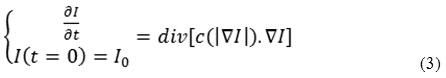
Where ∇ is the gradient operator which is used to identify the image’s edge as a step discontinuity in intensity; div is the divergence operator,| | represents the magnitude, c(x) is the diffusion coefficient, and I₀ is the initial image. Further the authors recommended application of 2 co-efficients:

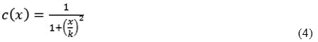
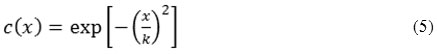
Where k is a parameter for edge magnitude. If

resulting in an all-pass filter. And, if

resulting in an isotropic filtering i.e. gaussian filtering. A discrete form of (1) is denoted by:

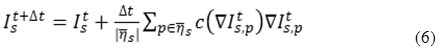
Where

the discretely sampled image, s is is the pixel position in a discrete 2D grid, Δt is the time step size,

is the spatial neighborhood of s,

is the number of pixels in the window.

The main benefits of AD are intra-region smoothing and edge maintenance. AD achieves the results extremely good for images that are tainted by additive noise [13]. Also, this method is preferred because of its low computational complexity [15]. Some developments for despeckling have been explained in the literature for ultrasound images. For the analysis of noise performance, we will employ the Teaching-Learning Based Optimization algorithm.

Harmony Search Algorithm

Harmony search algorithm is a powerful technique of metaheuristic analysis. This algorithm is based on the concept of music and harmonies for the purpose of optimization and can be used in conjunction with other algorithms like particle swarm optimization and likes of it [16].

This algorithm works on the analogy between music and optimization. Just like the music is aimed to have perfect state of harmony, an optimization process searches for perfect optimality of the process. To create a perfect harmony, the pitch, the timbre and the amplitude are to be created and adjusted perfectly. Thus, a skilled musician improvises a piece of music by either of the three option stated as follows:

Play a famous piece of music which the musician has already in his memory.

Play something similar to a famous piece of music

Compose a totally fresh, new and random notes.

All these three can be applied to the optimization process and are known as harmony memory utilization, adjusting of pitch and randomization respectively to yield the final optimized solution.

In this optimization technique, the utilization of harmony memory serves the same purpose as choice of the best fit individual while using the genetic algorithm. Further, for the optimization, the pitch is adjusted. Here, the usual method is linear adjustment of the pitch which is preferred over nonlinear adjustments which can also be adopted in certain cases. When considering genetic algorithm, pitch generation can be compared to the function of mutation. Also, for the process of pitch adjusting, the rate of pitch adjustment is defined which would help in the exploration of the optimal solution which may be lying scattered in the solution space. The rate of pitch adjustment is kept at a value of 0.1 to 0.5 in most practical cases so as to reach to the solution with the help of harmony search algorithm at a faster pace.

Also, coming to the final part of the HSA which is randomization, helps explore the entire global solution space which was not explore in the case of pitch adjustment resulting only in local exploration. This helps reach to the solution with desired accuracy and in a faster period of time.

Teaching-Learning Based Optimization Algorithm

Teaching–Learning-Based Optimization (TLBO) algorithm [18][19][20] reproduces the teaching–learning classroom environment where the students learn from their teachers in order to educate themselves. This algorithm does not necessitate algorithm-specific parameters, rather it needs common controlling parameters such as the population size and number of generations for its operation. TLBO is a population-based algorithm, in which the learners are contemplated to be the population and the subjects taught are similar to the design variables of the optimization problem. The outcome of the learners are corresponding to the fitness value of the optimization problem. The most suitable answer in the whole population is regarded as the teacher.

The algorithm reproduces 2 phases in the teaching-learning environment, i.e. Teacher phase and Learner phase.

Teacher Phase

In this phase, the main focus is on the teacher who imparts knowledge to the students in order to obtain a good performance from the students. Let there be x number of subjects which are similar to the design variables, and y number of learners. At a consecutive teaching-learning cycle i, M_j,i is the average performance of the learners in a particular subject ‘j’ (j = 1, 2, . . . , x). As a teacher is the highly experienced and knowledgeable in a subject, the algorithm regards the teacher as the best learner in the whole classroom.  In view of this detail, the difference between the performance of the teacher and the average performance of the learners in each subject is stated as:

Where X _j,kbest,i is the teacher’s performance, T_F is the teaching factor that is responsible for changing the value of mean and it can be either 1 or 2, r_i is the random number in [0,1]. The value of T_F is selected randomly with equal probability as:

Founded on the Difference _{Mean j,i} the current solution is revised in the teacher phase as per the below equation:

Where

is the updated value of  X _j,k,i.

Learner Phase

In this phase the learning part is reproduced wherein the learners learn by means of interaction between each other. A learner can learn more if the other learners are more knowledgeable than him or her. The learning phase is depicted as below:

Randomly pick 2 learners, A and B, such that

where

and

are the revised values of  X_total-A,l and X_total-B,l after the teacher’s phase is completed. For maximization problems, the below equations can be used.

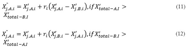
TLBO helps to unravel multi-dimensional, linear and nonlinear problems with substantial proficiency. Therefore the main objective for this research is to reduce the noising in the ultrasound images for accurate diagnosis.

Related Studies

Medical images are normally of less contrast and noise thereby having extremely low clarity attributed to the conditions and environments they are being taken. Denoising of ultrasound images is a challenging process relative to the other medical images that contain noise and artifacts, however ultrasound images additionally may comprise of blurring of edges [32].

As per Benazarti and Amiri [5], speckle noise persistently increases and has uneven frequencies that fluctuate continually. Thus the authors chose the logarithmic transformation as an ideal preference to transform signal-dependent rather a merely multiplicative noise to an additive noise. This research employs diffusion tensor which is required to acclimatize the flow diffusion in the direction of the indigenous orientation by executing anisotropic diffusion with the course of logical structure of stimulating features in the image. The authors have evidently depicted the efficacy of the algorithm.

Another research [1] developed denoising filters in the spatial domain by implementing the multi-scale transforms. The findings of the denoising process show that the spatial filters are smoothing the boundaries and lines in the ultrasound images. The researchers have used wavelet transform based methods that reduced the smoothing process; however, the boundaries remain undistinguished. Even though the wavelet transform performed well, the computation cost was high. The dual tree complex wavelet transforms and the double density dual tree complex wavelet transforms are doing extremely well in the elimination of speckle noise relative to the spatial filtering and multi-scale transform.

Andria et al [21] used the linear filtering of only the vertical and diagonal particulars of the ultrasound image. The information is acquired by means of first-level 2-D wavelet decomposition; despite the fact that the linear filtering is implemented using a Gaussian filter that has a kernel size. The size of the Gaussian filter relies upon the amplitude of the speckle noise. The final outcome was compared with distinctive linear and nonlinear denoising techniques. The research evidently showed that the proposed methodology was efficient and applicable to the real-world medical diagnosis.

De Fontes et al [23] developed an efficient real-time denoising model of ultrasound images which was an improvement of the NL-means method which is established on a non-local standard, i.e., the reinstated intensity of a pixel that is a mean that is complete because of all pixels in the image were adequate by the length between the patches [24]. The modified model includes an ultrasound dedicated noise model, and a GPU application of the proposed system. The findings suggest that this approach is effective for denoising the image and can be used in the real-time medical diagnosis. The computation time of this model for medium sized images, was less than 20ms.

Another denoising method [24] uses dual methods to eliminate the speckle noise and differentiate between a specific entity and the residual image. The first method consists of Block based Hard Thresholding (BHT) and Block based Soft Thresholding (BST) on pixels in wavelet domain wherein the actual ultrasound image is segregated into non-Overlapping blocks having dimensions 8, 16, 32 and 64. The next method comprises of rebuilding of the entity’s edges and texture with adaptive wavelet fusion. The Edges were dropped due to the distorting impact due to the previous method. Fusion rule and wavelet decomposition level are constituted to be adaptive for all the blocks by means of gradient histograms with Normalized Differential Mean (NDF) to present a maximum level of contrast between the denoised pixels and the entity pixels in the subsequent image. The 2 methods are termed as adaptive NDF block fusion with hard and soft thresholding (ANBF-HT and ANBF-ST). The graphic quality of the ultrasound image by this approach was enhanced.

Ranjani and Chitra [28] have recommended the application of a dual tree complex wavelet transform-based Levy Shrink algorithm (DTCWT) for denoising ultrasound images. The authors in their study employed this algorithm to eliminate speckle noise wherein the DTCWT coefficients of all the sub-bands are showed expending a substantially tracked Levy distribution.  By manipulating the observational miniscule instants of the ultrasound images comprising of noise along with the miniscule instants of the Levy and the Gaussian distribution, they ascertained the scale parameter of the Levy distribution by means of a closed-form expression. Finally they instigated a Bayesian MAP estimator to measure the coefficients.

A completely data-driven extension algorithm was proposed [29] for denoising ultrasound. The authors employed the hyperbolic wavelet method wherein the transform of the image prior to implementing multi-scale variance stabilization process by means of a Fisz transformation. Measuring the noise variance by means of an isotonic Nadaraya-Watson estimator, the proposed algorithm acclimatizes the wavelet coefficients statistics to the wavelet thresholding standard. The application of hyperbolic wavelets promises to improve the quality of the image in the same time, relating to the anisotropic characteristics of the important specifics.

Fredj and Malek [30] proposed a video restoration method by the application of a dedicated filter in order to modify the filter of anisotropic diffusion to the characteristics of the multiplicative noise present in the ultrasound video. The authors designed the system to lessen the processing time execution of the diffusion function employing parallel processors as a result of the optimization of the Graphics processor unit (GPU). The system employs the kuan diffusion function that has been implied on an individual image instigated on a standard CPU processor.

As per Wen and Qi [31], an image enhancement and denoising technique has been applied which is centered on wavelet analysis theory and fuzzy theory. The logarithmic transform, transform multiplicative noise into additive noise, and multi-scale wavelet transform were applied to the ultrasound images to obtain higher frequency and lower frequency wavelet coefficients. While the lower frequency coefficient was improved through the fuzzy method, the higher frequency coefficients were improved by the wavelet soft threshold denoising.

Experimental

Results and Discussions

For the purpose of this analysis, we obtained the data sets from a medical database available on the internet [26][27]. This data set is fed into the MATLAB platform and the original images of two of the ultrasounds of the liver of different patients are shown in Figure 1 and Figure 2

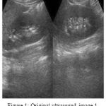Figure 1: Original ultrasound image 1   Click here to View figure

 

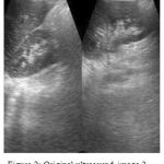Figure 2: Original ultrasound image 2   Click here to View figure

HSV stands for Hue, Saturation and Value. This parameter delineated colors i.e. hue or tint in relation to their shade i.e. saturation or quantity of grayness and their brightness value. The corresponding HSV of the unfiltered images are shown in figure 3 and figure 4.

Figure 3: HSV of original image 1   Click here to View figure

 

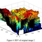Figure 4: HSV of original image 2   Click here to View figure

HSV separates luminosity, image intensity, color information and removes shadows. The distinct factors of HSV are explained below [25]

Hue is depicted as a number between 0 to 360 degrees signifying hues of red that begin at 0, yellow that begin at 60), green that begin at 120, cyan that begin at 180, blue that begin at 240 and magenta that begin at 300.

Saturation is the quantity of gray scale in the color from 0-100 per cent.

Value operates in combination with saturation and defines the brightness of the color from 0-100 per cent.

For the processof denoising in the ADF, diffusion function and discrete PDE solution are the parameters evaluated i=for the proper functioning of the said filter. After the denoising of the images using AD, the result with denoised images is shown is figure 5 and figure 6.

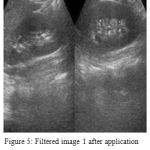Figure 5: Filtered image 1 after application of Anisotropic Diffusion     Click here to View figure

 

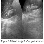Figure 6: Filtered image 2 after application of Anisotropic Diffusion   Click here to View figure

The corresponding HSV of the filtered images are shown in figure 7 and figure 8 respectivley.

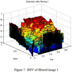Figure 7:  HSV of filtered image 1   Click here to View figure

 

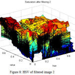Figure 8: HSV of filtered image 2   Click here to View figure

The function for converting RGB colormap into HSV colormap is given in MATLAB as: H = rgb2hsv(M) converts an RGB colormap M to an HSV colormap H. Both colormaps are m-by-3 matrices. The elements of both colormaps are in the range 0 to 1[33]

As deduced from the above images, it is evident that the denoising is efficiently carried out with a better HSV and reduced noise factor. We introduced Teaching–learning based optimization (TLBO) algorithm to evaluate the noise performance as the image may perhaps look the same even after filtering. TLBO helps in avoiding this confusion. TLBO algorithm is capable of performing the performance analysis on a range of standard unrestrained benchmark functions having dissimilar features.

By assigning the TLBO with the boundaries of the filter function, it is able to calculate the noise. Hence, the initial population is assigned to the algorithm as per figure 9 and the final population after TBLO is shown in figure 10. Also the time consumption of the entire process is depicted in figure 11 which gives an idea of the time response of the proposed technique.

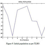Figure 9: Initial population as per TLBO   Click here to View figure

 

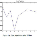Figure 10: Final population after TBLO   Click here to View figure

 

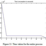Figure 11: Time taken for the entire process   Click here to View figure

The figure 12 and figure 13 depict the noise factor for image 1 and image 2 respectively.

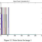Figure 12: Noise factor for image 1   Click here to View figure

 

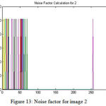Figure 13: Noise factor for image 2   Click here to View figure

The noise analysis carried out by TLBO is shown in figure 14 which was about 0.0063.

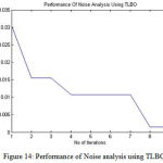Figure 14: Performance of Noise analysis using TLBO   Click here to View figure

 

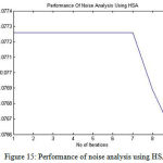Figure 15: Performance of noise analysis using HSA   Click here to View figure

 

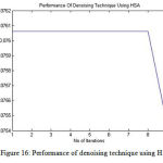Figure 16: Performance of denoising technique using HSA   Click here to View figure

The noise factor of the images (figure 12 and figure 13) clearly prove that the proposed method considerably reduces the noise in the images. However, using TLBO, it was also found that the images were over-filtered i.e. alongside the elimination of the noise some part of the image data possibly will also be removed (See figure 5 and figure 6), thus obtaining over-filtered images that do not give accuracy for carrying out an efficient diagnosis. Noise factor is the ratio of definite output noise to that which would persist if the device itself did not present noise. The corresponding noise performance analysis is depicted in figure 14.

A similar process is undertaken using the HSA for the purpose of optimization. The results of performance of noise and denoising are shown in figure 15 and figure 16.

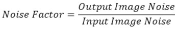
To analyze the percentage of noise for an image, we must calculate the noise factor which is the ratio of output image noise power to input image noise i.e. the noise subsequent to the filtering process and the noise present before the filtering techniques.

In comparison to other methods [1][5][21][23][26], the filtered image in figure 5 and figure 6 display better improvement of the ultrasound images with a considerably superior edges and an effective restraining of noise. The diffusion sufficiently monitors the course of the curvature lines.

Despite the denoising effectively carried out, the major drawback of this approach was that over-filtering of the ultrasound images was done and some amount of image data was lost. However, this work can be further enhanced in future by eliminating the over-filtering problem.

Conclusion

With age being a less determinant factor of diseases these days, there is an increased necessity to develop methods to be able to provide accurate diagnosis in order to detect the condition in its initial stages. Imaging modalities are susceptible to noise and thus require denoising of the images for clear diagnosis. Ultrasound is an efficient and beneficial imaging modality that helps in diagnosing muscle related disorders. For the purpose of denoising the speckle noise from the ultrasound images, we have adopted Anisotropic Diffusion for denoising of the image. This paper provides additionally the performance analysis of the denoising mechanism using the TLBO algorithm as well as HSA and a comparative study is undertaken for the same.

From various results, it can be concluded that the TLBO proposed in this paper is much more effecticve as compared to the performance of the HSA. While the proposed system is considered to be effective, the performance of the denoising was carried out by the TLBO algorithm to find that the denoising was over-filtering the image with the additional loss of data. Optimization of the current method is recommended to eliminate the problem of over-filtering of the data in the ultrasound image.

References

1. Prudhvi Raj V.N., Venkateswarlu T., Denoising of Medical Ultrasound Images using Spatial Filtering and Multiscale Transforms, International Journal of Computer Science & Information Technology (IJCSIT), Vol 4, No 6, December 2012.
2. Clague J E, Roberts N, Gibson H and Edwards R H, Muscle imaging in health and disease. Neuromuscular Disorder. 5 (3), 1995, 171-178.
   CrossRef
3. N. K, Anil A.R, Rajesh R., Digital image denoising in medical ultrasound images: a survey, ICGST AIML-11 Conference, Dubai, UAE, 2011, pp 12-14.
4. Abbott J.G, Thurstone F. L., Acoustic speckle: Theory and experimental analysis, Ultrasonic Imaging, 1979, Vol. 1, pp 303–324.
   CrossRef
5. Faouzi Benzarti, Hamid Amiri, Speckle Noise Reduction in Medical Ultrasound Images, IJCSI International Journal of Computer Science Issues, Vol. 9, Issue 2, No 3, March 2012.
6. A, Goal J., Malik S., Choudhary K., Deepika, Despeckling of Medical Ultrasound Images using Wiener Filter and Wavelet Transform, IJECT, 2011.
7. Sudha S., Suresh G.R, Sukanesh R., Speckle Noise Reduction in Ultrasound Images by Wavelet Thresholding based on Weighted Variance, International Journal of Computer Theory and Engineering, Vol. 1, 2009, pp 1793-8201.
   CrossRef
8. Loupas T., Mcdicken W., Allan P. L., An adaptive weighted median filter for speckle suppression in medical ultrasonic images, IEEE Transaction Circuits System, Vol. 36 (1), 1989, pp 129–135 .
   CrossRef
9. Taya P.C., Acton S. T., Hossack J. A., A wavelet thresholding method to reduce ultrasound artifacts, Computerized Medical Imaging and Graphics 35, 2011, pp 42–50.
   CrossRef
10. Frost V.S, Stiles J.A, Shanmugam K.S, Holtzman J.C., A model for radar image & its application To Adaptive digital filtering for multiplicative noise, IEEE Transaction on Pattern Analysis and Machine Intelligence, 1982, pp 175-165.
    CrossRef
11. Lee J.S., Digital image enhancement and noise filtering by using local statistics, IEEE Trans. Pattern Analysis and Machine Intelligence,
12. Kaun D.T, Sowchauk T., Strand C., Chavel P., Adaptive noise smoothing filters for signal dependent Noise, IEEE Transaction on pattern analysis and machine intelligence, Vol. 7, 1985, pp 165-177.
13. Yongjian Yu and Scott T. Acton, Speckle Reducing Anisotropic Diffusion, IEEE Transactions on Image Processing, Vol. 11, No. 11, November 2002.
14. Perona and J. Malik, Scale space and edge detection using anisotropic diffusion, IEEE Transaction on Pattern Analysis. Machine Intelligence, vol. 12, 1990, pp. 629–639.
    CrossRef
15. Chourmouzios Tsiotsios, Maria Petrou, On the choice of the parameters for anisotropic diffusion in image processing, Pattern Recognition (2012), http://dx.doi.org/10.1016/j.patcog.2012.11.012
    CrossRef
16. Yang, Xin-She. “Harmony search as a metaheuristic algorithm.” Music-inspired harmony search algorithm. Springer Berlin Heidelberg, 2009. 1-14.
17. Venkata Rao R., Vivek Patel, An improved teaching-learning-based optimization algorithm for solving unconstrained optimization problems, Transactions D: Computer Science & Engineering and Electrical Engineering, Scientia Iranica D, 20 (3), 2013, 710–720.
18. Rao R.V., Savsani V.J. Vakharia D.P., Teaching–learning-based optimization: a novel method for constrained mechanical design optimization problems, Computer Aided Design, 43(3), 2011, pp. 303–315.
    CrossRef
19. Rao R.V., Savsani V.J., Vakharia D.P., Teaching–learning-based optimization: a novel optimization method for continuous non-linear large scale problems, Information Science, 183(1), 2011, pp. 1–15.
    CrossRef
20. Rao R.V., Patel V., An elitist teaching–learning-based optimization algorithm for solving complex constrained optimization problems, International Journal of Industrial Engineering and Computing, 3(4), 2012, pp. 535–560.
    CrossRef
21. Andria G., Attivissimo F., Cavone G., Giaquinto N., Lanzolla A.M.L., Linear filtering of 2-D wavelet coefficients for denoising ultrasound medical images, Measurement 45, 2012, pp. 1792–1800.
    CrossRef
22. Antoni Buades, Bartomeu Coll, Jean-Michel Morel. A review of image denoising algorithms, with a new one, SIAM Journal on Multiscale Modeling and Simulation: A SIAM Interdisciplinary Journal, 4 (2), 2005, pp.490-530.
23. Fernanda Palhano Xavier de Fontes, Guillermo Andrade Barroso, Pierre Hellier. Real time ultrasound image denoising, Journal of Real-Time Image Processing, Springer Verlag, 6 (1), 2010, pp.15-22.
    CrossRef
24. Kishore P.V.V., Mallika K.L., Prasad M.V.D., Narayana K.L., Denoising Ultrasound Medical Images with Selective Fusion in Wavelet Domain, Second International Symposium on Computer Vision and the Internet, Procedia Computer Science 58, 2015, pp 129 – 139.
    CrossRef
25. Jacci Howard Bear, HSV, Published on 31^st October 2016, Available at http://desktoppub.about.com/od/glossary/g/HSV.htm
26. Ultrasound Images, Ultrasound images of diseases of the liver, Accessed on 21^st December 2016, Available at http://www.ultrasound-images.com/liver/
27. Online Medical Images, Ultrasound Images, Accessed on 21^st December 2016, Available at http://www.onlinemedicalimages.com/index.php/en/site-map
28. Ranjani J. and C. M. S., Bayesian denoising of ultrasound images using heavy-tailed Levy distribution, IET Image Processing, vol. 9, no. 4, pp. 338-345, 4 2015.
29. Farouj; J. M. Freyermuth; L. Navarro; M. Clausel; P. Delachartre, Hyperbolic Wavelet-Fisz denoising for a model arising in Ultrasound Imaging, IEEE Transactions on Computational Imaging , vol. no. 99, pp.1-1
30. H. Fredj and J. Malek, Real time ultrasound image denoising using NVIDIA CUDA, 2016 2nd International Conference on Advanced Technologies for Signal and Image Processing (ATSIP), Monastir, 2016, pp. 136-140.
31. Wen and W. Qi, “Enhancement and Denoising Method of Medical Ultrasound Image Based on Wavelet Analysis and Fuzzy Theory,” 2015 Seventh International Conference on Measuring Technology and Mechatronics Automation, Nanchang, 2015, pp. 448-452.
    CrossRef
32. Kaur, G. Singh and P. Kaur, “Image enhancement of ultrasound images using multifarious denoising filters and GA,” 2016 International Conference on Advances in Computing, Communications and Informatics (ICACCI), Jaipur, 2016, pp. 2375-2384.
    CrossRef
33. MATLAB Documentation – MathWorks India, Available at http://in.mathworks.com/help/matlab/.

(Visited 1,255 times, 1 visits today)